

Learning action-oriented models through active inference
Open accessPublished version of a preprint
The DOI matches its Crossref record; 83 of the 84 references it cites were found in a registry or an index, and 1 are not checked yet.
Abstract
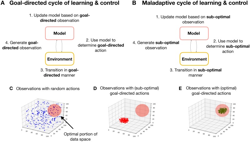
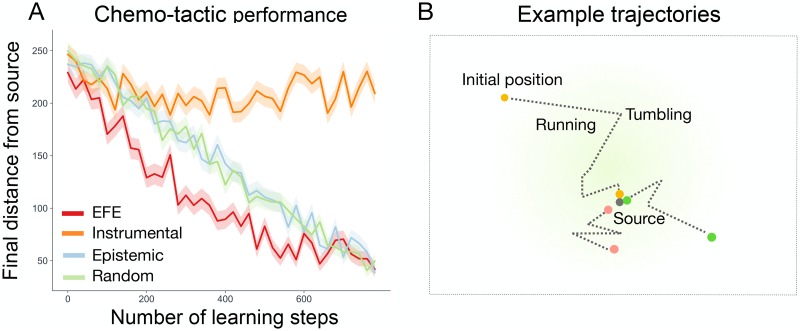
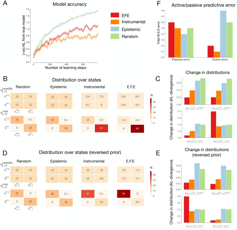
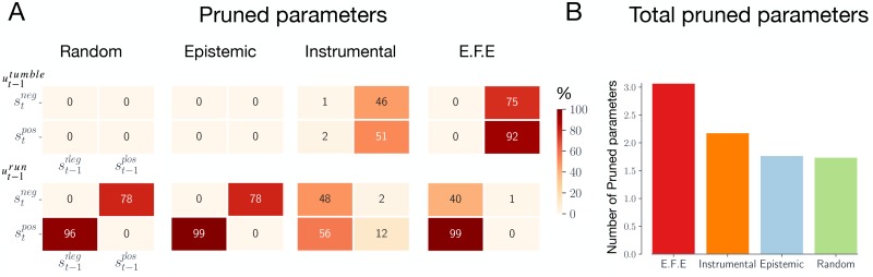
Converging theories suggest that organisms learn and exploit probabilistic models of their environment. However, it remains unclear how such models can be learned in practice. The open-ended complexity of natural environments means that it is generally infeasible for organisms to model their environment comprehensively. Alternatively, action-oriented models attempt to encode a parsimonious representation of adaptive agent-environment interactions. One approach to learning action-oriented models is to learn online in the presence of goal-directed behaviours. This constrains an agent to behaviourally relevant trajectories, reducing the diversity of the data a model need account for. Unfortunately, this approach can cause models to prematurely converge to sub-optimal solutions, through a process we refer to as a bad-bootstrap. Here, we exploit the normative framework of active inference to show that efficient action-oriented models can be learned by balancing goal-oriented and epistemic (information-seeking) behaviours in a principled manner. We illustrate our approach using a simple agent-based model of bacterial chemotaxis. We first demonstrate that learning via goal-directed behaviour indeed constrains models to behaviorally relevant aspects of the environment, but that this approach is prone to sub-optimal convergence. We then demonstrate that epistemic behaviours facilitate the construction of accurate and comprehensive models, but that these models are not tailored to any specific behavioural niche and are therefore less efficient in their use of data. Finally, we show that active inference agents learn models that are parsimonious, tailored to action, and which avoid bad bootstraps and sub-optimal convergence. Critically, our results indicate that models learned through active inference can support adaptive behaviour in spite of, and indeed because of, their departure from veridical representations of the environment. Our approach provides a principled method for learning adaptive models from limited interactions with an environment, highlighting a route to sample efficient learning algorithms.
Overview
The claims and statistics of this paper haven’t been checked yet.
Free: it reads the open-access text and checks the first 5 claims that cite a source we can check. Create a free account to check every claim.
Integrity signals
Registry
Cites
Statistics
Figures

Verification
Claims the paper makes
The claims and statistics of this paper haven’t been checked yet.
Free: it reads the open-access text and checks the first 5 claims that cite a source we can check. Create a free account to check every claim.
Claims other papers make about this one
Each is checked against this paper’s own text: does it say what the citing paper says it does?
The source backs part of the claim, not all of it — or backs it for a different population, condition or comparison.
In the citing paper
“This unique formulation of confirmation bias as an epistemic phenomenon helps explain how individuals continuously forage their environment for information, but may become stuck in a so-called ‘bad bootstrap’ that simply reinforces existing beliefs about the world, which in the face of new information may lead to sub-optimal behaviour [131].”
From Epistemic Communities under Active Inference (2022) · cites this paper as [131]
Experimental — accuracy not yet measured
Self-check
Percentages, sums and reported differences re-computed from the paper’s own numbers.
The self-check needs the paper’s full text.
Citations
Cites
The Ecological Approach to Visual Perception: Classic Edition
Gibson, J. J. (2014) · doi:10.4324/9781315740218 · Cited by 12,132
Playing Atari with Deep Reinforcement Learning
Mnih, V., Kavukcuoglu, K., Silver, D., Graves, A., Antonoglou, I., Wierstra, D., & Riedmiller, M. (2013) · arXiv · doi:10.48550/arxiv.1312.5602 · Cited by 9,471
The free-energy principle: a unified brain theory?
Friston, K. (2010) · Nature Reviews Neuroscience · doi:10.1038/nrn2787 · Cited by 8,120 · cited 1×
“Active inference is a normative theory that unifies perception, action and learning under a single imperative—the minimization of variational free energy [42, 43].”
BackgroundMarkov decision processes: Discrete stochastic dynamic programming
Hazeghi, K., & Puterman, M. L. (1995) · Journal of the American Statistical Association · doi:10.2307/2291177 · Cited by 8,037
Markov Decision Processes: Discrete Stochastic Dynamic Programming
Puterman, M. L. (1994) · Wiley Series in Probability and Statistics · doi:10.1002/9780470316887 · Cited by 6,024
Rao, R. P. N., & Ballard, D. H. (1999) · Nature Neuroscience · doi:10.1038/4580 · Cited by 5,483 · cited 2×
“This casts perception as a process of approximate inference, connecting active inference to influential theories such as the Bayesian brain hypothesis (Knill and Pouget, 2004; Gregory, 1980) and predictive coding (Rao and Ballard, 1999).”
MethodBengio, Y., Louradour, J., Collobert, R., & Weston, J. (2009) · Proceedings of the 26th Annual International Conference on Machine Learning · doi:10.1145/1553374.1553380 · Cited by 5,366
Watkins, C. (1989) · OpenGrey (Institut de l'Information Scientifique et Technique) · doi:10.17863/cam.132164 · Cited by 5,297
The Bayesian brain: The role of uncertainty in neural coding and computation
Knill, D. C., & Pouget, A. (2004) · Trends in Neurosciences · doi:10.1016/j.tins.2004.10.007 · Cited by 2,588
Chemotaxis in Escherichia coli analysed by Three-dimensional Tracking
BERG, H. C., & BROWN, D. A. (1972) · Nature · doi:10.1038/239500a0 · Cited by 2,231
Every good regulator of a system must be a model of that system †
CONANT, R. C., & ROSS ASHBY, W. (1970) · International Journal of Systems Science · doi:10.1080/00207727008920220 · Cited by 1,063
Keeping the neural networks simple by minimizing the description length of the weights
Hinton, G. E., & van Camp, D. (1993) · Proceedings of the sixth annual conference on Computational learning theory - COLT '93 · doi:10.1145/168304.168306 · Cited by 994 · cited 12×
“It is therefore an (expected) KL-divergence between posterior and prior beliefs, a quantity known as (expected) Bayesian surprise (Baldi and Itti, 2010).”
MethodInfluentialDolan, R. J., & Dayan, P. (2013) · Neuron · doi:10.1016/j.neuron.2013.09.007 · Cited by 977
Transfer learning using computational intelligence: A survey
Lu, J., Behbood, V., Hao, P., Zuo, H., Xue, S., & Zhang, G. (2015) · Knowledge-Based Systems · doi:10.1016/j.knosys.2015.01.010 · Cited by 968
The Ecological Approach to Visual Perception: Classic Edition
Gibson, J. J. (2014) · Cited by 896
A Survey on Policy Search for Robotics
Deisenroth, M. P. (2011) · Foundations and Trends in Robotics · doi:10.1561/2300000021 · Cited by 798
Gregory, R. L. (1980) · Philosophical Transactions of the Royal Society of London. B, Biological Sciences · doi:10.1098/rstb.1980.0090 · Cited by 789
Friston, K. (2013) · Journal of The Royal Society Interface · doi:10.1098/rsif.2013.0475 · Cited by 754 · cited 4×
“…and machine learning suggests that organisms achieve this feat by exploiting probabilistic models of their world (Doll et al., 2012; Dayan and Berridge, 2014; Botvinick and Weinstein, 2014; Dolan and Dayan, 2013; Conant and Ashby, 1970; Friston, 2013; Kuvayev and Sutton, 1996; Deisenroth, 2011).”
BackgroundInfluentialActive inference and epistemic value
Friston, K., Rigoli, F., Ognibene, D., Mathys, C., Fitzgerald, T., & Pezzulo, G. (2015) · Cognitive Neuroscience · doi:10.1080/17588928.2015.1020053 · Cited by 731
Every Good Regulator of a System Must Be a Model of That System
Conant, R. C., & Ashby, W. R. (1991) · Facets of Systems Science · doi:10.1007/978-1-4899-0718-9_37 · Cited by 712
Friston, K., FitzGerald, T., Rigoli, F., Schwartenbeck, P., O⿿Doherty, J., & Pezzulo, G. (2016) · Neuroscience & Biobehavioral Reviews · doi:10.1016/j.neubiorev.2016.06.022 · Cited by 674
Friston, K. J., & Stephan, K. E. (2007) · Synthese · doi:10.1007/s11229-007-9237-y · Cited by 673
Bayesian model reduction and empirical Bayes for group (DCM) studies
Friston, K. J., Litvak, V., Oswal, A., Razi, A., Stephan, K. E., van Wijk, B. C. M., Ziegler, G., & Zeidman, P. (2016) · NeuroImage · doi:10.1016/j.neuroimage.2015.11.015 · Cited by 599
Adaptive prediction of environmental changes by microorganisms
Mitchell, A., Romano, G. H., Groisman, B., Yona, A., Dekel, E., Kupiec, M., Dahan, O., & Pilpel, Y. (2009) · Nature · doi:10.1038/nature08112 · Cited by 581
Survey of Model-Based Reinforcement Learning: Applications on Robotics
Polydoros, A. S., & Nalpantidis, L. (2017) · Journal of Intelligent & Robotic Systems · doi:10.1007/s10846-017-0468-y · Cited by 534
Deep reinforcement learning in a handful of trials using probabilistic dynamics models
Chua, K., Calandra, R., McAllister, R., & Levine, S. (2018) · arXiv · doi:10.48550/arxiv.1805.12114 · Cited by 525 · cited 2×
“A significant drawback to existing methods is that they tend to prematurely converge to sub-optimal solutions [33].”
MethodTowards a neuroscience of active sampling and curiosity
Gottlieb, J., & Oudeyer, P.-Y. (2018) · Nature Reviews Neuroscience · doi:10.1038/s41583-018-0078-0 · Cited by 494 · cited 1×
“Rather, organisms actively sample information from their environment, a process which plays an important role in both perception and learning (Yang et al., 2018; Gottlieb and Oudeyer, 2018; Lungarella and Sporns, 2005; Friston et al., 2012b).”
BackgroundMcKay, R. T., & Dennett, D. C. (2009) · Behavioral and Brain Sciences · doi:10.1017/s0140525x09990975 · Cited by 474
The Markov blankets of life: autonomy, active inference and the free energy principle
Kirchhoff, M., Parr, T., Palacios, E., Friston, K., & Kiverstein, J. (2018) · Journal of The Royal Society Interface · doi:10.1098/rsif.2017.0792 · Cited by 473
VIME: Variational Information Maximizing Exploration
Houthooft, R., Chen, X., Duan, Y., Schulman, J., Turck, F. D., & Abbeel, P. (2016) · arXiv (Cornell University) · doi:10.48550/arxiv.1605.09674 · Cited by 472
Perceptions as Hypotheses: Saccades as Experiments
Friston, K., Adams, R. A., Perrinet, L., & Breakspear, M. (2012) · Frontiers in Psychology · doi:10.3389/fpsyg.2012.00151 · Cited by 462 · cited 1×
“Rather, organisms actively sample information from their environment, a process which plays an important role in both perception and learning (Yang et al., 2018; Gottlieb and Oudeyer, 2018; Lungarella and Sporns, 2005; Friston et al., 2012b).”
BackgroundReinforcement learning or active inference?
Friston, K. J., Daunizeau, J., & Kiebel, S. J. (2009) · PLoS ONE · doi:10.1371/journal.pone.0006421 · Cited by 443
Large-Scale Study of Curiosity-Driven Learning
Burda, Y., Edwards, H., Pathak, D., Storkey, A., Darrell, T., & Efros, A. A. (2018) · arXiv · doi:10.48550/arxiv.1808.04355 · Cited by 401 · cited 1×
“…models to determine epistemic (or intrinsic, information-seeking, uncertainty reducing ) actions that attempt to minimize the model uncertainty in a directed manner (Stadie et al., 2015; Houthooft et al., 2016; Sun et al., 2011; Friston et al., 2015; Burda et al., 2018; Friston et al., 2017).”
BackgroundBruineberg, J., Kiverstein, J., & Rietveld, E. (2018) · Synthese · doi:10.1007/s11229-016-1239-1 · Cited by 383 · cited 1×
“The arguments and simulations presented in this paper resonate with previous work which views an active inference agent as a ‘crooked scientist’ [76, 77].”
The ubiquity of model-based reinforcement learning
Doll, B. B., Simon, D. A., & Daw, N. D. (2012) · Current Opinion in Neurobiology · doi:10.1016/j.conb.2012.08.003 · Cited by 380
Being a Beast Machine: The Somatic Basis of Selfhood
Seth, A. K., & Tsakiris, M. (2018) · Trends in Cognitive Sciences · doi:10.1016/j.tics.2018.08.008 · Cited by 371
Self-citationThe free energy principle for action and perception: A mathematical review
Buckley, C. L., Kim, C. S., McGregor, S., & Seth, A. K. (2017) · Journal of Mathematical Psychology · doi:10.1016/j.jmp.2017.09.004 · Cited by 363
Self-citationModel-based and model-free Pavlovian reward learning: Revaluation, revision, and revelation
Dayan, P., & Berridge, K. C. (2014) · Cognitive, Affective, & Behavioral Neuroscience · doi:10.3758/s13415-014-0277-8 · Cited by 357 · cited 1×
“Converging research in neuroscience, biology, and machine learning suggests that organisms achieve this feat by exploiting probabilistic models of their world (Doll et al., 2012; Dayan and Berridge, 2014; Botvinick and Weinstein, 2014; Dolan and Dayan, 2013; Conant and Ashby, 1970; Friston, 2013; Kuvayev and Sutton, 1…”
BackgroundActive Inference, Curiosity and Insight
Friston, K. J., Lin, M., Frith, C. D., Pezzulo, G., Hobson, J. A., & Ondobaka, S. (2017) · Neural Computation · doi:10.1162/neco_a_00999 · Cited by 351
Mapping Information Flow in Sensorimotor Networks
Lungarella, M., & Sporns, O. (2006) · PLoS Computational Biology · doi:10.1371/journal.pcbi.0020144 · Cited by 293
The anatomy of choice: dopamine and decision-making.
Friston, K., Schwartenbeck, P., FitzGerald, T., Moutoussis, M., Behrens, T., & Dolan, R. J. (2014) · Philosophical Transactions of the Royal Society B: Biological Sciences · doi:10.1098/rstb.2013.0481 · Cited by 289
Incentivizing Exploration In Reinforcement Learning With Deep Predictive Models
Stadie, B. C., Levine, S., & Abbeel, P. (2015) · arXiv (Cornell University) · doi:10.48550/arxiv.1507.00814 · Cited by 280
Computational mechanisms of curiosity and goal-directed exploration
Schwartenbeck, P., Passecker, J., Hauser, T. U., FitzGerald, T. H., Kronbichler, M., & Friston, K. J. (2019) · eLife · doi:10.7554/elife.41703 · Cited by 254
A comparison of direct and model-based reinforcement learning
Atkeson, C. G., & Santamaria, J. C. (2002) · Proceedings of International Conference on Robotics and Automation · doi:10.1109/robot.1997.606886 · Cited by 239
The cybernetic Bayesian brain : from interoceptive inference to sensorimotor contingencies
Seth, A. K. (2015) · MIND Group · doi:10.25358/openscience-84 · Cited by 239
Self-citationDeep temporal models and active inference
Friston, K. J., Rosch, R., Parr, T., Price, C., & Bowman, H. (2017) · Neuroscience & Biobehavioral Reviews · doi:10.1016/j.neubiorev.2017.04.009 · Cited by 237
Generalised free energy and active inference
Parr, T., & Friston, K. J. (2019) · Biological Cybernetics · doi:10.1007/s00422-019-00805-w · Cited by 236 · cited 2×
“inference assigns a higher posterior probability to the control states that are expected to 164 minimize free energy [52].”
BackgroundBenchmarking Model-Based Reinforcement Learning
Wang, T., Bao, X., Clavera, I., Hoang, J., Wen, Y., Langlois, E., Zhang, S., Zhang, G., Abbeel, P., & Ba, J. (2019) · arXiv · doi:10.48550/arxiv.1907.02057 · Cited by 226
Environmentally mediated synergy between perception and behaviour in mobile robots
Verschure, P. F. M. J., Voegtlin, T., & Douglas, R. J. (2003) · Nature · doi:10.1038/nature02024 · Cited by 216
Seth, A. K. (2015) · Figshare · doi:10.15502/9783958570108 · Cited by 211
Self-citationClark, A. (2015) · The Southern Journal of Philosophy · doi:10.1111/sjp.12120 · Cited by 202
Model-based hierarchical reinforcement learning and human action control
Botvinick, M., & Weinstein, A. (2014) · Philosophical Transactions of the Royal Society B Biological Sciences · doi:10.1098/rstb.2013.0480 · Cited by 186
Theoretical perspectives on active sensing
Yang, S. C., Wolpert, D. M., & Lengyel, M. (2016) · Current Opinion in Behavioral Sciences · doi:10.1016/j.cobeha.2016.06.009 · Cited by 157
Planning to be surprised: optimal bayesian exploration in dynamic environments
Sun, Y., Gomez, F., & Schmidhuber, J. (2011) · Lecture notes in computer science · doi:10.1007/978-3-642-22887-2_5 · Cited by 134 · cited 3×
“…models to determine epistemic (or intrinsic, information-seeking, uncertainty reducing ) actions that attempt to minimize the model uncertainty in a directed manner (Stadie et al., 2015; Houthooft et al., 2016; Sun et al., 2011; Friston et al., 2015; Burda et al., 2018; Friston et al., 2017).”
BackgroundPredictive Processing and the Representation Wars
Williams, D. (2018) · Minds and Machines · doi:10.1007/s11023-017-9441-6 · Cited by 134
Autonomy and Enactivism: Towards a Theory of Sensorimotor Autonomous Agency
Barandiaran, X. E. (2017) · Topoi · doi:10.1007/s11245-016-9365-4 · Cited by 128
Bacteria are not too small for spatial sensing of chemical gradients: An experimental evidence
Thar, R., & Kühl, M. (2003) · Proceedings of the National Academy of Sciences · doi:10.1073/pnas.1030795100 · Cited by 120
Deep temporal models and active inference
Friston, K. J., Rosch, R., Parr, T., Price, C., & Bowman, H. (2018) · Neuroscience & Biobehavioral Reviews · doi:10.1016/j.neubiorev.2018.04.004 · Cited by 119 · cited 2×
“However, the active inference scheme described in this paper has a degree of biological plausibility [54], and there is some evidence to suggest that bacteria engage in model-based behaviours [55–58].”
BackgroundWhere There is Life There is Mind: In Support of a Strong Life-Mind Continuity Thesis
Kirchhoff, M. D., & Froese, T. (2017) · Entropy · doi:10.3390/e19040169 · Cited by 114 · cited 1×
“…embodied and enactive approaches (Kiverstein, 2018; Kirchhoff and Robertson, 2018; Ramstead et al., 2019; Negru, 2018; Linson et al., 2018; Pezzulo et al., 2017; Clark, 2015; Williams, 2018; Kirchhoff Michael et al., 2018; Kirchhoff and Froese, 2017; Friston, 2013; Baltieri and Buckley, 2019a,c,b).”
BackgroundFree-energy minimization in joint agent-environment systems: A niche construction perspective
Bruineberg, J., Rietveld, E., Parr, T., van Maanen, L., & Friston, K. J. (2018) · Journal of Theoretical Biology · doi:10.1016/j.jtbi.2018.07.002 · Cited by 99
Enactivism and predictive processing: a non-representational view
Kirchhoff, M. D., & Robertson, I. (2018) · Philosophical Explorations · doi:10.1080/13869795.2018.1477983 · Cited by 94
Information Self-Structuring: Key Principle for Learning and Development
Lungarella, M., & Sporns, O. (2005) · Proceedings. The 4nd International Conference on Development and Learning, 2005. · doi:10.1109/devlrn.2005.1490938 · Cited by 92
Linson, A., Clark, A., Ramamoorthy, S., & Friston, K. (2018) · Frontiers in Robotics and AI · doi:10.3389/frobt.2018.00021 · Cited by 90
Reliable misrepresentation and tracking theories of mental representation
Mendelovici, A. (2012) · Philosophical Studies · doi:10.1007/s11098-012-9966-8 · Cited by 75
Modeling habits as self-sustaining patterns of sensorimotor behavior
Egbert, M. D., & Barandiaran, X. E. (2014) · Frontiers in Human Neuroscience · doi:10.3389/fnhum.2014.00590 · Cited by 69
What is value—accumulated reward or evidence?
Friston, K., Adams, R., & Montague, R. (2012) · Frontiers in Neurorobotics · doi:10.3389/fnbot.2012.00011 · Cited by 67
Beyond Homeostasis: A Predictive-Dynamic Framework for Understanding Cellular Behavior
Freddolino, L., & Tavazoie, S. (2012) · Annual Review of Cell and Developmental Biology · doi:10.1146/annurev-cellbio-092910-154129 · Cited by 65 · cited 1×
“, 2018), and there is some evidence to suggest that bacteria engage in model-based behaviours (Mitchell et al., 2009; Mitchell and Lim, 2016; Freddolino and Tavazoie, 2012) (7)The chemical gradient is computed spatially rather than temporally (Thar and Kuhl, 2003), and thus only depends on the agent’s current position…”
BackgroundAction is enabled by systematic misrepresentations
Wiese, W. (2017) · Erkenntnis · doi:10.1007/s10670-016-9867-x · Cited by 60
Free Energy and the Self: An Ecological–Enactive Interpretation
Kiverstein, J. (2020) · Topoi · doi:10.1007/s11245-018-9561-5 · Cited by 54
An active inference implementation of phototaxis
Baltieri, M., & Buckley, C. L. (2017) · European Conference on Artificial Life · doi:10.7551/ecal_a_011 · Cited by 51
Self-citationModel-Based Approaches to Active Perception and Control
Pezzulo, G., Donnarumma, F., Iodice, P., Maisto, D., & Stoianov, I. (2017) · Entropy · doi:10.3390/e19060266 · Cited by 45
A Theory of Cheap Control in Embodied Systems
Montúfar, G., Ghazi-Zahedi, K., & Ay, N. (2015) · PLoS Computational Biology · doi:10.1371/journal.pcbi.1004427 · Cited by 33
Mitchell, A., & Lim, W. A. (2016) · BioEssays · doi:10.1002/bies.201600090 · Cited by 27
Generalised free energy and active inference: can the future cause the past?Preprint
Parr, T., & Friston, K. J. (2018) · bioRxiv (Cold Spring Harbor Laboratory) · doi:10.1101/304782 · Cited by 24
Generative models as parsimonious descriptions of sensorimotor loops
Baltieri, M., & Buckley, C. L. (2019) · Behavioral and Brain Sciences · doi:10.1017/s0140525x19001353 · Cited by 21
Self-citationEpistemological Dimensions of Evolutionary Psychology
Breyer, T. (2014) · Springer eBooks · doi:10.1007/978-1-4939-1387-9 · Cited by 20
The dark room problem in predictive processing and active inference, a legacy of cognitivism?
Baltieri, M., & Buckley, C. L. (2019) · Conference on Artificial Life (ALIFE) · doi:10.1162/isal_a_00137 · Cited by 19
Self-citationNonmodular Architectures of Cognitive Systems based on Active Inference
Baltieri, M., & Buckley, C. L. (2019) · International Joint Conference on Neural Networks (IJCNN) · doi:10.1109/ijcnn.2019.8852048 · Cited by 13
Self-citationNonmodular architectures of cognitive systems based on active inference
Baltieri, M., & Buckley, C. L. (2019) · Sussex Research Online (University of Sussex) · Cited by 10
Self-citationA measure of good motor actions for active visual perception
Ruesch, J., Ferreira, R. P. M., & Bernardino, A. J. M. (2011) · IEEE International Conference on Development and Learning (ICDL) · doi:10.1109/devlrn.2011.6037355 · Cited by 8
Gauging the value of good data: Informational embodiment quantification
Thornton, C. (2010) · Adaptive Behavior · doi:10.1177/1059712310383914 · Cited by 6
SELF-ORGANIZATION, AUTOPOIESIS, FREE-ENERGY PRINCIPLE AND AUTONOMY
Negru, T. (2018) · Organon F · Cited by 6
The dark room problem in predictive processing and active inference, a legacy of cognitivism?
Baltieri, M., & Buckley, C. L. (2019) · Conference on Artificial Life (ALIFE) · doi:10.1162/isal_a_00137.xml · Cited by 4
Self-citationWhen misrepresentations are successful
Zehetleitner, M., & Schönbrodt, F. D. (2015) · Cited by 2
Research works printed but not linked: 2
- Kuvayev L, Sutton RS. Model-Based Reinforcement Learning with an Approximate, Learned Model. In: in Proceedings of the Ninth Yale Workshop on Adaptive and Learning Systems; 1996. p. 101–105.
- Ha D, Schmidhuber J. World Models. arXiv:180310122. 2018;.
Cited by
A step-by-step tutorial on active inference and its application to empirical data
Smith, R., Friston, K. J., & Whyte, C. J. (2022) · Journal of Mathematical Psychology · doi:10.1016/j.jmp.2021.102632 · Cited by 246
Predictive processing as a systematic basis for identifying the neural correlates of consciousness
Hohwy, J., & Seth, A. (2020) · Philosophy and the Mind Sciences · doi:10.33735/phimisci.2020.ii.64 · Cited by 170
Self-citationThe Emperor's New Markov Blankets
Bruineberg, J., Dołęga, K., Dewhurst, J., & Baltieri, M. (2022) · Behavioral and Brain Sciences · doi:10.1017/s0140525x21002351 · Cited by 124
The evolution of brain architectures for predictive coding and active inference
Pezzulo, G., Parr, T., & Friston, K. (2022) · Philosophical Transactions of the Royal Society B · doi:10.1098/rstb.2020.0531 · Cited by 117
An Active Inference Approach to Modeling Structure Learning: Concept Learning as an Example Case
Smith, R., Schwartenbeck, P., Parr, T., & Friston, K. J. (2020) · Frontiers in Computational Neuroscience · doi:10.3389/fncom.2020.00041 · Cited by 99
Metadata
- Authors
- Tschantz, A., Seth, A. K., & Buckley, C. L.
- Affiliations
- University of Sussex (GB)
- Canadian Institute for Advanced Research (CA)
- Corresponding author
- Tschantz, Alexander
- Buckley, Christopher L.
- Venue
- PLOS Computational Biology
- Publisher
- Public Library of Science (PLoS)
- Published
- 2020-04-23
- Volume
- 16
- Issue
- 4
- Pages
- e1007805
- ISSN
- 1553-734X (ISSN-L)
- 1553-7358
- PMC
- PMC7200021
- OpenAlex
- W3017990858
- Semantic Scholar
- 6417d1bfc8f7dc8df7b04e50f8eb9188784b776a
- Cited by
- 121
- References
- 80
- Citations by year
- 2026: 8 · 2025: 25 · 2024: 9 · 2023: 9 · 2022: 23 · 2021: 31 · 2020: 16
- FWCI
- 10.61
- Type
- journal article
- Language
- en
- Update notices
- new_version (2020-05-05)
- Open access
- gold
- doi.org
- Licence
- Locations
- PLoS Computational Biology (publishedVersion, cc-by)
- PubMed Central (publishedVersion, cc-by)
- PubMed (publishedVersion)
- RePEc: Research Papers in Economics (submittedVersion)
- DOAJ (DOAJ: Directory of Open Access Journals) (submittedVersion, cc-by-sa)
- Figshare (submittedVersion, cc-by)
- Funders
- Canadian Institute for Advanced Research
- Biotechnology and Biological Sciences Research Council (BB/P022197/1)
- Topics
- Life Sciences › Neuroscience › Cognitive Neuroscience › Embodied and Extended Cognition
- Physical Sciences › Computer Science › Artificial Intelligence › Reinforcement Learning in Robotics
- Physical Sciences › Computer Science › Artificial Intelligence › Bayesian Modeling and Causal Inference
- Keywords
- active inference, Bayesian learning, goal-directed behavior, information seeking, model convergence, bacterial chemotaxis, sample efficiency, agent-environment interaction
- MeSH terms
- Algorithms, Chemotaxis, Environment, Goals, Learning, Models, Biological, Bacterial Physiological Phenomena, Computational Biology
About these checks
Registry, retraction, Cites and statistics results are computed, not judged, with one exception: a printed reference that no index lists is read once by a model before it counts as a citation error. Claims are extracted by a model and kept only when their quote appears verbatim in the text; each cited source is then checked, with a model’s help, for whether it says what the claim relies on. Those verdicts can be wrong — read the claim’s quote and the cited source before relying on one.
Statistics and arithmetic are recomputed, not judged.
Confidence bands are shown only for fields calibrated on our annotated test set. None is calibrated yet, so no band is shown.
What counts as a claim ›How we measure confidence ›How we check this ›
Are you an author, or do you see a problem with this page? Request a review
Data sources
Bibliographic data: Semantic Scholar, OpenAlex, Crossref.
Contains information from the Semantic Scholar Academic Graph Datasets, made available under the ODC Attribution License (ODC-BY 1.0).
Semantic Scholar’s data is described in: Kinney, R., et al. (2023). The Semantic Scholar Open Data Platform. arXiv:2301.10140.
