

Predicting cellular responses to complex perturbations in high‐throughput screens
Open accessThe DOI matches its Crossref record; 50 of the 50 references it cites were found in a registry or an index; 4 of the 18 sources its claims cite were checked for support.
Abstract
Recent advances in multiplexed single‐cell transcriptomics experiments facilitate the high‐throughput study of drug and genetic perturbations. However, an exhaustive exploration of the combinatorial perturbation space is experimentally unfeasible. Therefore, computational methods are needed to predict, interpret, and prioritize perturbations. Here, we present the compositional perturbation autoencoder (CPA), which combines the interpretability of linear models with the flexibility of deep‐learning approaches for single‐cell response modeling. CPA learns to in silico predict transcriptional perturbation response at the single‐cell level for unseen dosages, cell types, time points, and species. Using newly generated single‐cell drug combination data, we validate that CPA can predict unseen drug combinations while outperforming baseline models. Additionally, the architecture's modularity enables incorporating the chemical representation of the drugs, allowing the prediction of cellular response to completely unseen drugs. Furthermore, CPA is also applicable to genetic combinatorial screens. We demonstrate this by imputing in silico 5,329 missing combinations (97.6% of all possibilities) in a single‐cell Perturb‐seq experiment with diverse genetic interactions. We envision CPA will facilitate efficient experimental design and hypothesis generation by enabling in silico response prediction at the single‐cell level and thus accelerate therapeutic applications using single‐cell technologies.
Overview
CoChat Summary
TL;DR
The paper introduces the compositional perturbation autoencoder (CPA), a deep-learning model that learns disentangled, additive latent embeddings of perturbations and covariates to predict single-cell transcriptional responses to unseen drug, dose, time, species, and genetic combinations. CPA is validated on multiple public datasets and a newly generated drug-combination dataset, and extended by chemCPA to predict responses to completely unseen drugs using chemical descriptors.
Key findings
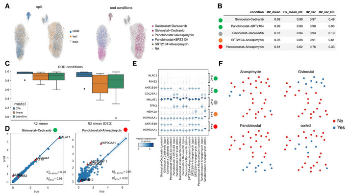
- CPA predicted unseen drug combinations in a new A549 combination dataset (combosciplex, n = 63,378 cells, 32 perturbation/combination conditions), including a held-out Panobinostat + Alvespimycin combination with an R2 of 0.81; it outperformed a random baseline and a linear model.
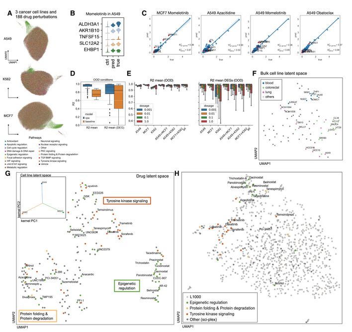
- On sci-Plex3 (n = 290,889 cells; 188 compounds; A549, K562, MCF7; four doses), CPA outperformed scGen by 1.54% on mean prediction and 35.85% on variance prediction, and learned drug embeddings that clustered compounds by mechanism, including epigenetic, tyrosine kinase signaling, and protein formation/degradation pathways.
- In a Perturb-seq genetic screen (108,497 cells; 284 conditions; 131 unique double-gene combinations), CPA imputed 5,329 missing combinations (97.6% of all possibilities); however, a simple baseline performed on par with CPA and linear models for mean whole-transcriptome prediction, suggesting limited nonlinear effects at that level.
- chemCPA, which incorporates chemical descriptors, improved prediction for unseen drugs and combinations; when single-drug Panobinostat observations were held out, median R2 on DEGs dropped from 0.85 to 0.38, but the single-drug Panobinostat effect could still be predicted with high accuracy.
Methods
- CPA is an autoencoder that encodes gene expression into a basal latent state, adversarially removes perturbation and covariate information from that state, then additively composes learned perturbation and covariate embeddings with nonlinear dose/time scalers before decoding to gene expression.
- The model was trained and evaluated on six public datasets plus a newly generated A549 drug-combination dataset; datasets included Kang et al. PBMCs, sci-Plex2, sci-Plex3, Hagai et al. cross-species LPS phagocytes, Norman et al. Perturb-seq, and L1000 bulk data.
- Evaluation used train/test/out-of-distribution splits, R2 on means and variances, Wasserstein distance, clustering metrics, and a distance-based uncertainty score; benchmarks included random baseline, linear baseline, and scGen.
Limitations
- The paper states that CPA will fail if test data are very different from training data, that predictions cannot replace experimental validation, and that the uncertainty score is a condition-level heuristic rather than a cell-specific or Bayesian uncertainty estimate.
- The paper notes that CPA is deterministic, uses gene expression alone, cannot directly capture post-transcriptional, signaling, or cell-communication effects, and may require systematic hyperparameter sweeping for best performance.
- The text makes evident that CPA cannot predict completely unseen drugs without an extension such as chemCPA, and that some held-out combinations, such as Alvespimycin + Panobinostat, showed distribution shifts that neither CPA nor chemCPA fully identified (R2 about 0.3 on DEGs).
Model-written summary. Check it against the paper before relying on it.
Integrity signals
Registry
Cites
Statistics
Figures



Verification
Claims the paper makes
4 Valid · 0 Not valid · 11 Not checked · 91 Own results and interpretations
The cited sources support only part of this claim — read each source’s verdict below.
In the paper
“We further evaluated CPA to predict a previously reported (Norman et al, 2019) genetic epistatic interaction between DUSP9 and ETS1, leading to domination of the DUSP9 phenotype in doubly perturbed cells (Fig 5C).”
§ Predicting cellular responses to complex perturbations in high‐throughput screens > Results > CPA allows modeling combinatorial genetic perturbations
What the sources say
- Partly supportedcites Norman et al, 2019 sourceExperimental — accuracy not yet measured
In “Ordering genes into linear pathways using Perturb-seq” (Fig. 5A; page not provided), the source reports that the DUSP9 phenotype dominated in a double perturbation, but the partner was ETS2, not ETS1. The sentence’s statement about what CPA predicted is the citing authors’ own result, not a finding attributed to this source. (LLM, conf=0.88)
plainstates a cause- Asserted: passes — The authors put it forward as true.
- Checkable: passes — It can be checked against evidence.
- Load-bearing: passes — The paper’s conclusions depend on it.
- Based: passes — The paper gives a reason why it holds.
- Partly supported
Every source the paper cites for this claim was checked and supports it.
In the paper
“Furthermore, we observed that chemCPA generalized particularly well for compounds that belonged to the histone deacetylation pathway (Fig 4C), which is in line with the original sci‐Plex publication (Srivatsan et al, 2020) and general support within this perturbation dataset.”
§ Predicting cellular responses to complex perturbations in high‐throughput screens > Results > CPA is an extensible framework for predicting single‐cell perturbations
What the sources say
- Supportedcites Srivatsan et al, 2020 source
The cited sci-Plex paper does not evaluate chemCPA; the citing authors present that as their own observation. The citation supports the stated alignment with sci-Plex: the Results section, “Inference of chemical and mechanistic properties of HDAC inhibitors” (page not available), identifies HDAC inhibitors as the most prominent compound-response group across three cell lines and describes a consensus response trajectory. (LLM, conf=0.87)
boostedstates an association- Asserted: passes — The authors put it forward as true.
- Checkable: passes — It can be checked against evidence.
- Load-bearing: unclear — It is unclear whether the paper’s conclusions depend on it.
- Based: passes — The paper gives a reason why it holds.
- Supported
Every source the paper cites for this claim was checked and supports it.
In the paper
“Overexpression of both CBL and CNN1 up‐regulate known gene markers (Norman et al, 2019) such as hemoglobins (see HBA1/2 and HBG1/2 in Fig 5B).”
§ Predicting cellular responses to complex perturbations in high‐throughput screens > Results > CPA allows modeling combinatorial genetic perturbations
What the sources say
- Supportedcites Norman et al, 2019 source
The section 'Constructing a GI manifold reveals biological processes driving GIs' (p. ~4) states that overexpression of CBL and CNN1 caused strong induction of canonical erythroid markers, specifically hemoglobin genes (6-39-fold), plus SLC25A37 and GYPA. This matches the claim that overexpressing CBL and CNN1 up-regulates known gene markers such as hemoglobins; the same passage also notes the effect in the HUDEP2 erythroid progenitor model. (LLM, conf=0.92)
plainstates a cause- Asserted: passes — The authors put it forward as true.
- Checkable: passes — It can be checked against evidence.
- Load-bearing: passes — The paper’s conclusions depend on it.
- Based: passes — The paper gives a reason why it holds.
- Supported
A result the paper states — it cites no source for it, so there is none to check. The quote shows it is in the paper.
In the paper
“Crucially, the latent representation that the CPA encoder learns about a cell's basal state is disentangled from (does not contain information about) the embeddings corresponding to the perturbation and the covariates.”
§ Predicting cellular responses to complex perturbations in high‐throughput screens > Results > Compositional perturbation autoencoder (CPA)
plain- Asserted: passes — The authors put it forward as true.
- Checkable: passes — It can be checked against evidence.
- Load-bearing: passes — The paper’s conclusions depend on it.
- Based: passes — The paper gives a reason why it holds.
- Rests on an assumption not shown here.
A result the paper reports from its own data — it cites no other source for it, so there is none to check. The quote shows it is in the paper.
In the paper
“Compositional perturbation autoencoder performs worse when predicting experiments with more unseen covariates.”
§ Predicting cellular responses to complex perturbations in high‐throughput screens > Results > CPA finds interpretable latent spaces in large‐scale single‐cell high‐throughput screens
plainstates a causen = 3- Asserted: passes — The authors put it forward as true.
- Checkable: passes — It can be checked against evidence.
- Load-bearing: passes — The paper’s conclusions depend on it.
- Based: passes — The paper gives a reason why it holds.
53 more claims
Create a free account to see all 106 claims and to verify the 12 references still open.
- It may state two separate claims as one. 37
- Probably not a substantial claim. 13
Claims other papers make about this one
Each is checked against this paper’s own text: does it say what the citing paper says it does?
The source backs part of the claim, not all of it — or backs it for a different population, condition or comparison.
In the citing paper
“There are a number of existing methods that perform perturbation-effect analysis in single-cell omics data, but none of them achieve guaranteed confounder identification, which is a necessary condition for interpretable causal-effect estimation.”
From Causal identification of single-cell experimental perturbation effects with CINEMA-OT (2023) · cites this paper as [23]
Experimental — accuracy not yet measuredThe check wasn’t confident either way, so it gives no verdict — never disputed.
In the citing paper
“We acknowledge a lack of strong correlation between the magnitude of PICALM alteration and its functional effects in CRISPR-engineered iMGs, probably due to technical variations in iMG differentiation and/or the nonlinear relationship between gene expression and cellular phenotypes due to epistasis and systems buffering54,55.”
From PICALM Alzheimer’s risk allele causes aberrant lipid droplets in microglia (2025) · cites this paper as [55]
Experimental — accuracy not yet measuredIn the citing paper
“An extension of CPA called chemCPA [54] introduces into the autoencoder architecture a perturbation network that encodes small molecules using their known chemical descriptors, thus enabling extrapolations to unseen drugs.”
From A mini-review on perturbation modelling across single-cell omic modalities (2024) · cites this paper as [54]
Self-check
Percentages, sums and reported differences re-computed from the paper’s own numbers.
Each contradiction between two passages listed here was confirmed by an independent check.
Rated minor: it would not touch a result — a value no result rests on, a p-value that stays on the same side of the significance level, or a conflict that is clerical, resolved elsewhere in the paper, or outside its own findings.
In the paper
“Using the same set of compounds tested in the sci‐Plex dataset together with 853 other compounds (for a total of 1,000 compounds)”
§ Predicting cellular responses to complex perturbations in high‐throughput screens > Results > CPA finds interpretable latent spaces in large‐scale single‐cell high‐throughput screens
Reported 1000 · recomputed 1041
Rated minor: it would not touch a result — a value no result rests on, a p-value that stays on the same side of the significance level, or a conflict that is clerical, resolved elsewhere in the paper, or outside its own findings.
In the paper
§ Predicting cellular responses to complex perturbations in high‐throughput screens > Materials and Methods > Methods and Protocols
“We generated a novel validation dataset of 32 samples containing combinations of 13 compounds selected from the 188 compounds in sci‐Plex 2 (Srivatsan et al, 2020).”
§ Predicting cellular responses to complex perturbations in high‐throughput screens > Results > CPA allows predictive and exploratory analyses of single‐cell perturbation experiments
“Sciplex2 from Srivatsan et al (2020) contains measurements of a human lung adenocarcinoma cell line (A549) treated with four drug perturbations at increasing dosages (Appendix Fig S4A).”
Rated minor: it would not touch a result — a value no result rests on, a p-value that stays on the same side of the significance level, or a conflict that is clerical, resolved elsewhere in the paper, or outside its own findings.
In the paper
§ Predicting cellular responses to complex perturbations in high‐throughput screens > Results > CPA finds interpretable latent spaces in large‐scale single‐cell high‐throughput screens
“UMAP representation of sci‐Plex samples (n = 290,889) of A549, K562, and MCF7 cell‐lines”
§ Predicting cellular responses to complex perturbations in high‐throughput screens > Materials and Methods > Methods and Protocols
“The data was subset to half its size, reducing it to 290,888 cells.”
Citations
Cites
(2008) · Journal of Machine Learning Research · Cited by 33,051
Distributed Representations of Words and Phrases and their Compositionality
Mikolov, T., Sutskever, I., Chen, K., Corrado, G., & Dean, J. (2013) · arXiv · doi:10.48550/arxiv.1310.4546 · Cited by 24,533 · cited 1×
“We introduce the CPA (see Materials and Methods), a method combining ideas from natural language processing (preprint: Mikolov et al , 2013) and computer vision (preprint: Radford et al , 2015; Lample et al , 2017) to predict the effects of combinations of perturbations on single-cell gene…”
MethodComprehensive Integration of Single-Cell Data
Stuart, T., Butler, A., Hoffman, P., Hafemeister, C., Papalexi, E., Mauck, W. M., Hao, Y., Stoeckius, M., Smibert, P., & Satija, R. (2019) · Cell · doi:10.1016/j.cell.2019.05.031 · Cited by 15,453
Advances in Neural Information Processing Systems 29
Teymur, O., Zygalakis, K., & Calderhead, B. (2016) · Cited by 13,887
Unsupervised representation learning with deep convolutional generative adversarial networks
Radford, A., Metz, L., & Chintala, S. (2015) · arXiv · doi:10.48550/arxiv.1511.06434 · Cited by 12,235 · cited 1×
“…introduce the CPA (see Materials and Methods), a method combining ideas from natural language processing (preprint: Mikolov et al , 2013) and computer vision (preprint: Radford et al , 2015; Lample et al , 2017) to predict the effects of combinations of perturbations on single-cell gene expression.”
MethodUMAP: Uniform Manifold Approximation and Projection
McInnes, L., Healy, J., Saul, N., & Großberger, L. (2018) · Journal of Open Source Software · doi:10.21105/joss.00861 · Cited by 9,826
SCANPY: large-scale single-cell gene expression data analysis
Wolf, F. A., Angerer, P., & Theis, F. J. (2018) · Genome Biology · doi:10.1186/s13059-017-1382-0 · Cited by 8,881
Self-citationUMAP: Uniform Manifold Approximation and Projection for Dimension Reduction
McInnes, L., Healy, J., & Melville, J. (2018) · arXiv · doi:10.48550/arxiv.1802.03426 · Cited by 7,101
Deep generative modeling for single-cell transcriptomics
Lopez, R., Regier, J., Cole, M. B., Jordan, M. I., & Yosef, N. (2018) · Nature Methods · doi:10.1038/s41592-018-0229-2 · Cited by 2,530
Slide-seq: A scalable technology for measuring genome-wide expression at high spatial resolution
Rodriques, S. G., Stickels, R. R., Goeva, A., Martin, C. A., Murray, E., Vanderburg, C. R., Welch, J., Chen, L. M., Chen, F., & Macosko, E. Z. (2019) · Science · doi:10.1126/science.aaw1219 · Cited by 2,424
CUT&Tag for efficient epigenomic profiling of small samples and single cells
Kaya-Okur, H. S., Wu, S. J., Codomo, C. A., Pledger, E. S., Bryson, T. D., Henikoff, J. G., Ahmad, K., & Henikoff, S. (2019) · Nature Communications · doi:10.1038/s41467-019-09982-5 · Cited by 2,187
Ancient DNA and the rewriting of human history: be sparing with Occam’s razor
Haber, M., Mezzavilla, M., Xue, Y., & Tyler-Smith, C. (2016) · Genome Biology · doi:10.1186/s13059-015-0866-z · Cited by 1,924
Dixit, A., Parnas, O., Li, B., Chen, J., Fulco, C. P., Jerby-Arnon, L., Marjanovic, N. D., Dionne, D., Burks, T., Raychowdhury, R., et al. (2016) · Cell · doi:10.1016/j.cell.2016.11.038 · Cited by 1,863 · cited 4×
“To study such genetic interactions (GIs), recent perturbation scRNA-seq assays allow us to measure the gene expression response of a cell to the perturbation of genes alone or in combination (Dixit et al , 2016; Datlinger et al , 2017).”
BackgroundInfluentialA single-cell transcriptomic atlas characterizes ageing tissues in the mouse
The Tabula Muris Consortium, Almanzar, N., Antony, J., Baghel, A. S., Bakerman, I., Bansal, I., Barres, B. A., Beachy, P. A., Berdnik, D., Bilen, B., et al. (2020) · Nature · doi:10.1038/s41586-020-2496-1 · Cited by 1,247
Multiplexed droplet single-cell RNA-sequencing using natural genetic variation
Kang, H. M., Subramaniam, M., Targ, S., Nguyen, M., Maliskova, L., McCarthy, E., Wan, E., Wong, S., Byrnes, L., Lanata, C. M., et al. (2018) · Nature Biotechnology · doi:10.1038/nbt.4042 · Cited by 1,101 · cited 3×
“We first demonstrated the performance and functionality of the CPA on three small single-cell datasets: a dataset of PBMCs stimulated with IFN-β (Kang et al , 2018), a dataset of human lung cancer cells perturbed by four drugs (Srivatsan et al , 2020), and a longitudinal cross-species dataset of lipopolysaccharide (LP…”
MethodInfluentialPooled CRISPR screening with single-cell transcriptome readout.
Datlinger, P., Rendeiro, A. F., Schmidl, C., Krausgruber, T., Traxler, P., Klughammer, J., Schuster, L. C., Kuchler, A., Alpar, D., & Bock, C. (2017) · Nature Methods · doi:10.1038/nmeth.4177 · Cited by 1,096 · cited 2×
“To study such genetic interactions (GIs), recent perturbation scRNA-seq assays allow us to measure the gene expression response of a cell to the perturbation of genes alone or in combination (Dixit et al , 2016; Datlinger et al , 2017).”
BackgroundConstruction of a human cell landscape at single-cell level
Han, X., Zhou, Z., Fei, L., Sun, H., Wang, R., Chen, Y., Chen, H., Wang, J., Tang, H., Ge, W., et al. (2020) · Nature · doi:10.1038/s41586-020-2157-4 · Cited by 1,087
Single-cell RNA-seq denoising using a deep count autoencoder
Eraslan, G., Simon, L. M., Mircea, M., Mueller, N. S., & Theis, F. J. (2019) · Nature Communications · doi:10.1038/s41467-018-07931-2 · Cited by 1,084 · cited 2×
“Although we opted to implement a deterministic autoencoder scheme, extensions toward variational models (Lopez et al , 2018; Lotfollahi et al , 2020), as well as cost functions other than mean squared error (Eraslan et al , 2019) are straightforward.”
MethodSelf-citationCombinatorial drug therapy for cancer in the post-genomic era
Al-Lazikani, B., Banerji, U., & Workman, P. (2012) · Nature Biotechnology · doi:10.1038/nbt.2284 · Cited by 1,070
Mechanisms of drug combinations: interaction and network perspectives
Jia, J., Zhu, F., Ma, X., Cao, Z. W., Li, Y. X., & Chen, Y. Z. (2009) · Nature Reviews Drug Discovery · doi:10.1038/nrd2683 · Cited by 969
High-throughput sequencing of the transcriptome and chromatin accessibility in the same cell
Chen, S., Lake, B. B., & Zhang, K. (2019) · Nature Biotechnology · doi:10.1038/s41587-019-0290-0 · Cited by 810 · cited 1×
“…network-based approaches, CPA could be extended to include other modalities, for example via multimodal single-cell CRISPR (Frangieh et al , 2021; Papalexi et al , 2021) combined scRNA-seq and ATAC-seq (Clark et al , 2018; Chen et al , 2019) and CUT&Tag (Kaya-Okur et al , 2019; Wu et al , 2021).”
Dissecting cell identity via network inference and in silico gene perturbation
Kamimoto, K., Stringa, B., Hoffmann, C. M., Jindal, K., Solnica-Krezel, L., & Morris, S. A. (2023) · Nature · doi:10.1038/s41586-022-05688-9 · Cited by 677
scGen predicts single-cell perturbation responses
Lotfollahi, M., Wolf, F. A., & Theis, F. J. (2019) · Nature Methods · doi:10.1038/s41592-019-0494-8 · Cited by 661
Self-citationClark, S. J., Argelaguet, R., Kapourani, C.-A., Stubbs, T. M., Lee, H. J., Alda-Catalinas, C., Krueger, F., Sanguinetti, G., Kelsey, G., Marioni, J. C., et al. (2018) · Nature Communications · doi:10.1038/s41467-018-03149-4 · Cited by 657 · cited 2×
“However, due to the flexibility of neural network-based approaches, CPA could be extended to include other modalities, for example via multimodal single-cell CRISPR (Frangieh et al , 2021; Papalexi et al , 2021) combined scRNA-seq and ATAC-seq (Clark et al , 2018; Chen et al , 2019) and CUT&Tag (Kaya-Okur et al , 2019…”
MULTI-seq: sample multiplexing for single-cell RNA sequencing using lipid-tagged indices
McGinnis, C. S., Patterson, D. M., Winkler, J., Conrad, D. N., Hein, M. Y., Srivastava, V., Hu, J. L., Murrow, L. M., Weissman, J. S., Werb, Z., et al. (2019) · Nature Methods · doi:10.1038/s41592-019-0433-8 · Cited by 643
The Human Cell Atlas: from vision to reality
Rozenblatt-Rosen, O., Stubbington, M. J. T., Regev, A., & Teichmann, S. A. (2017) · Nature · doi:10.1038/550451a · Cited by 638
Mapping single-cell data to reference atlases by transfer learning
Lotfollahi, M., Naghipourfar, M., Luecken, M. D., Khajavi, M., Büttner, M., Wagenstetter, M., Avsec, Ž., Gayoso, A., Yosef, N., Interlandi, M., et al. (2022) · Nature Biotechnology · doi:10.1038/s41587-021-01001-7 · Cited by 602
Self-citationMater, A. C., & Coote, M. L. (2019) · Journal of Chemical Information and Modeling · doi:10.1021/acs.jcim.9b00266 · Cited by 565 · cited 1×
“These could, for example, be the similarity of chemical compounds (Mater & Coote, 2019), or clinical-covariate induced differences of patient IDs.”
BackgroundMachine learning approaches to drug response prediction: challenges and recent progress
Adam, G., Rampášek, L., Safikhani, Z., Smirnov, P., Haibe-Kains, B., & Goldenberg, A. (2020) · npj Precision Oncology · doi:10.1038/s41698-020-0122-1 · Cited by 425
Single-cell and spatial transcriptomics reveal somitogenesis in gastruloids
van den Brink, S. C., Alemany, A., van Batenburg, V., Moris, N., Blotenburg, M., Vivié, J., Baillie-Johnson, P., Nichols, J., Sonnen, K. F., Martinez Arias, A., et al. (2020) · Nature · doi:10.1038/s41586-020-2024-3 · Cited by 404
Massively multiplex chemical transcriptomics at single-cell resolution
Srivatsan, S. R., McFaline-Figueroa, J. L., Ramani, V., Saunders, L., Cao, J., Packer, J., Pliner, H. A., Jackson, D. L., Daza, R. M., Christiansen, L., et al. (2020) · Science · doi:10.1126/science.aax6234 · Cited by 401
Self-citationA human cell atlas of fetal chromatin accessibility
Domcke, S., Hill, A. J., Daza, R. M., Cao, J., O’Day, D. R., Pliner, H. A., Aldinger, K. A., Pokholok, D., Zhang, F., Milbank, J. H., et al. (2020) · Science · doi:10.1126/science.aba7612 · Cited by 400
Self-citationExploring genetic interaction manifolds constructed from rich single-cell phenotypes
Norman, T. M., Horlbeck, M. A., Replogle, J. M., Ge, A. Y., Xu, A., Jost, M., Gilbert, L. A., & Weissman, J. S. (2019) · Science · doi:10.1126/science.aax4438 · Cited by 392 · cited 9×
“Headers indicate gene-wise regression coefficients, and interaction mode suggested by (Norman et al , 2019 ).”
BackgroundMethodInfluentialMenden, M. P., Wang, D., Mason, M. J., Szalai, B., Bulusu, K. C., Guan, Y., Yu, T., Kang, J., Jeon, M., Wolfinger, R., et al. (2019) · Nature Communications · doi:10.1038/s41467-019-09799-2 · Cited by 363
Frangieh, C. J., Melms, J. C., Thakore, P. I., Geiger-Schuller, K. R., Ho, P., Luoma, A. M., Cleary, B., Jerby-Arnon, L., Malu, S., Cuoco, M. S., et al. (2021) · Nature Genetics · doi:10.1038/s41588-021-00779-1 · Cited by 276
Papalexi, E., Mimitou, E. P., Butler, A. W., Foster, S., Bracken, B., Mauck, W. M., Wessels, H.-H., Hao, Y., Yeung, B. Z., Smibert, P., et al. (2021) · Nature Genetics · doi:10.1038/s41588-021-00778-2 · Cited by 237 · cited 1×
“…network-based approaches, CPA could be extended to include other modalities, for example via multimodal single-cell CRISPR (Frangieh et al , 2021; Papalexi et al , 2021) combined scRNA-seq and ATAC-seq (Clark et al , 2018; Chen et al , 2019) and CUT&Tag (Kaya-Okur et al , 2019; Wu et al , 2021).”
Gene expression variability across cells and species shapes innate immunity
Hagai, T., Chen, X., Miragaia, R. J., Rostom, R., Gomes, T., Kunowska, N., Henriksson, J., Park, J.-E., Proserpio, V., Donati, G., et al. (2018) · Nature · doi:10.1038/s41586-018-0657-2 · Cited by 220
Single-cell CUT&Tag analysis of chromatin modifications in differentiation and tumor progression
Wu, S. J., Furlan, S. N., Mihalas, A. B., Kaya-Okur, H. S., Feroze, A. H., Emerson, S. N., Zheng, Y., Carson, K., Cimino, P. J., Keene, C. D., et al. (2021) · Nature Biotechnology · doi:10.1038/s41587-021-00865-z · Cited by 201
Kim, K.-T., Lee, H. W., Lee, H.-O., Song, H. J., Jeong, D. E., Shin, S., Kim, H., Shin, Y., Nam, D.-H., Jeong, B. C., et al. (2016) · Genome Biology · doi:10.1186/s13059-016-0945-9 · Cited by 198 · cited 1×
“These shortcomings become more apparent when exploring the effects of combination therapies (Al-Lazikani et al , 2012; Kim et al , 2016; Sachs et al , 2020) or genetic perturbations (Dixit et al , 2016; Datlinger et al , 2017; Norman et al , 2019), where the experimental screening of all possible…”
BackgroundDr.VAE: improving drug response prediction via modeling of drug perturbation effects
Rampášek, L., Hidru, D., Smirnov, P., Haibe-Kains, B., & Goldenberg, A. (2019) · Bioinformatics · doi:10.1093/bioinformatics/btz158 · Cited by 179
Targeted pharmacological therapy restores β-cell function for diabetes remission
Sachs, S., Bastidas-Ponce, A., Tritschler, S., Bakhti, M., Böttcher, A., Sánchez-Garrido, M. A., Tarquis-Medina, M., Kleinert, M., Fischer, K., Jall, S., et al. (2020) · Nature Metabolism · doi:10.1038/s42255-020-0171-3 · Cited by 147
Self-citationFröhlich, F., Kessler, T., Weindl, D., Shadrin, A., Schmiester, L., Hache, H., Muradyan, A., Schütte, M., Lim, J.-H., Heinig, M., et al. (2018) · Cell Systems · doi:10.1016/j.cels.2018.10.013 · Cited by 143
Self-citationOptimized single-nucleus transcriptional profiling by combinatorial indexing
Martin, B. K., Qiu, C., Nichols, E., Phung, M., Green-Gladden, R., Srivatsan, S., Blecher-Gonen, R., Beliveau, B. J., Trapnell, C., Cao, J., et al. (2023) · Nature Protocols · doi:10.1038/s41596-022-00752-0 · Cited by 133
Self-citationConditional out-of-distribution generation for unpaired data using transfer VAE
Lotfollahi, M., Naghipourfar, M., Theis, F. J., & Wolf, F. A. (2020) · Bioinformatics · doi:10.1093/bioinformatics/btaa800 · Cited by 130 · cited 3×
“Aside from CPA, existing methods (Lotfollahi et al , 2020; Russ-kikh et al , 2020) such as scGen (Lotfollahi et al , 2019) have also been shown capable of predicting single-cell perturbation responses when the dataset contains no combinatorial treatment or dose-dependent perturbations.”
BackgroundMethodSelf-citationYuan, B., Shen, C., Luna, A., Korkut, A., Marks, D. S., Ingraham, J., & Sander, C. (2021) · Cell Systems · doi:10.1016/j.cels.2020.11.013 · Cited by 125
Highly multiplexed single-cell RNA-seq by DNA oligonucleotide tagging of cellular proteins
Gehring, J., Hwee Park, J., Chen, S., Thomson, M., & Pachter, L. (2020) · Nature Biotechnology · doi:10.1038/s41587-019-0372-z · Cited by 122 · cited 2×
“OOD prediction would enable the study of perturbations in the presence of different treatment doses (Hagai et al , 2018; Srivatsan et al , 2020), combination therapies (Gehring et al , 2020), multiple genetic knockouts (Norman et al , 2019), and changes across time (Hagai et al , 2018).”
BackgroundSingle-cell genomic approaches for developing the next generation of immunotherapies
Yofe, I., Dahan, R., & Amit, I. (2020) · Nature Medicine · doi:10.1038/s41591-019-0736-4 · Cited by 114
Enhancing scientific discoveries in molecular biology with deep generative models
Lopez, R., Gayoso, A., & Yosef, N. (2020) · Molecular Systems Biology · doi:10.15252/msb.20199198 · Cited by 82
Russkikh, N., Antonets, D., Shtokalo, D., Makarov, A., Vyatkin, Y., Zakharov, A., & Terentyev, E. (2020) · Bioinformatics · doi:10.1093/bioinformatics/btaa624 · Cited by 21
Systems Pharmacogenomic Landscape of Drug Similarities from LINCS data: Drug Association Networks
Musa, A., Tripathi, S., Dehmer, M., Yli-Harja, O. P., Kauffman, S. A., & Emmert‐Streib, F. (2019) · Scientific Reports · doi:10.1038/s41598-019-44291-3 · Cited by 17
Research works printed but not linked: 6
- Gal Y, Ghahramani Z (2016) Dropout as a bayesian approximation: representing model uncertainty in deep learning. In International Conference on Machine Learning, pp 1050–1059. PMLR
- Goodfellow I, Bengio Y, Courville A, Bengio Y (2016) Deep learning. Cambridge: MIT Press
- Hetzel L, Böhm S, Kilbertus N, Günnemann S, Lotfollahi M, Theis FJ (2022) Predicting cellular responses to novel drug perturbations at a single‐cell resolution. In NeurIPS 2022
- Landrum G (2006) RDKit: Open source cheminformatics https://www.rdkit.org
- Sohn K, Lee H, Yan X (2015) Learning structured output representation using deep conditional generative models. In Advances in Neural Information Processing Systems 28, Cortes C, Lawrence ND, Lee DD, Sugiyama M, Garnett R (eds), pp 3483–3491. New York, NY: Curran Associates, Inc
- Zhao J, Kim Y, Zhang K, Rush A, LeCun Y (2018) Adversarially regularized autoencoders. In International Conference on Machine Learning, pp 5902–5911. PMLR
Cited by
scGPT: Towards Building a Foundation Model for Single-Cell Multi-omics Using Generative AI
Cui, H., Wang, C., Maan, H., Pang, K., Luo, F., & Wang, B. (2023) · doi:10.1101/2023.04.30.538439 · Cited by 1,694
“We conducted a performance comparison between scGPT and two other recent methods, GEARS [38] and CPA [39].”
MethodInfluentialBest practices for single-cell analysis across modalities
Heumos, L., Schaar, A. C., Lance, C., Litinetskaya, A., Drost, F., Zappia, L., Lücken, M. D., Strobl, D. C., Henao, J., Curion, F., et al. (2023) · Nature Reviews Genetics · doi:10.1038/s41576-023-00586-w · Cited by 1,051
Self-citationLarge-scale foundation model on single-cell transcriptomics
Hao, M., Gong, J., Zeng, X., Liu, C., Guo, Y., Cheng, X., Wang, T., Ma, J., Zhang, X., & Song, L. (2024) · Nature Methods · doi:10.1038/s41592-024-02305-7 · Cited by 628
How to build the virtual cell with artificial intelligence: Priorities and opportunities
Bunne, C., Roohani, Y., Rosen, Y., Gupta, A., Zhang, X., Roed, M., Alexandrov, T., AlQuraishi, M., Brennan, P., Burkhardt, D. B., et al. (2024) · Cell · doi:10.1016/j.cell.2024.11.015 · Cited by 393
Self-citationPredicting transcriptional outcomes of novel multigene perturbations with GEARS
Roohani, Y., Huang, K., & Leskovec, J. (2024) · Nature Biotechnology · doi:10.1038/s41587-023-01905-6 · Cited by 355
“GEARS functionalizes this graph-based inductive bias using a graph neural network (GNN) architecture 33 .”
Metadata
- Authors
- Lotfollahi, M., Klimovskaia Susmelj, A., De Donno, C., Hetzel, L., Ji, Y., Ibarra, I. L., Srivatsan, S. R., Naghipourfar, M., Daza, R. M., Martin, B., Shendure, J., McFaline‐Figueroa, J. L., Boyeau, P., Wolf, F. A., Yakubova, N., Günnemann, S., Trapnell, C., Lopez‐Paz, D., & Theis, F. J.
- Affiliations
- Wellcome Sanger Institute (GB)
- Helmholtz Munich (DE)
- University of Washington (US)
- University of California, Berkeley (US)
- Howard Hughes Medical Institute (US)
- Technical University of Munich (DE)
- Corresponding author
- Theis, Fabian J
- ORCID
- Venue
- Molecular Systems Biology
- Published
- 2023-05-08
- Volume
- 19
- Issue
- 6
- Pages
- e11517-e11517
- ISSN
- 1744-4292 (ISSN-L)
- PMC
- PMC10258562
- OpenAlex
- W4375955255
- Cited by
- 307
- References
- 50
- Citations by year
- 2026: 118 · 2025: 97 · 2024: 71 · 2023: 19
- FWCI
- 26.94
- Type
- journal article
- Language
- en
- Open access
- gold
- doi.org
- Licence
- other-oa
- creativecommons.org/licenses/by/4.0/ (tdm)
- creativecommons.org/licenses/by/4.0/ (vor)
- Locations
- Molecular Systems Biology (publishedVersion, other-oa)
- PubMed Central (publishedVersion, cc-by)
- PubMed (publishedVersion)
- eScholarship (California Digital Library) (submittedVersion, other-oa)
- DOAJ (DOAJ: Directory of Open Access Journals) (submittedVersion, cc-by-sa)
- PuSH - Publication Server of Helmholtz Zentrum München (submittedVersion, cc-by)
- Funders
- Bundesministerium für Bildung und Forschung (L031L0214A, 01IS18036A, 01IS18053A)
- Chan Zuckerberg Initiative (2018‐182835, 2019‐207271)
- EC | Horizon 2020 Framework Programme (874656)
- Helmholtz Association (ZT‐I‐0007, ZT‐I‐PF‐5‐01)
- Topics
- Life Sciences › Biochemistry, Genetics and Molecular Biology › Molecular Biology › Single-cell and spatial transcriptomics
- Life Sciences › Biochemistry, Genetics and Molecular Biology › Molecular Biology › Gene Regulatory Network Analysis
- Life Sciences › Pharmacology, Toxicology and Pharmaceutics › Drug Discovery › Computational Drug Discovery Methods
- Keywords
- single-cell transcriptomics, Perturb-seq, chemical representation
- MeSH terms
- Single-Cell Gene Expression Analysis, Computational Biology, Gene Expression Profiling, High-Throughput Screening Assays
About these checks
Registry, retraction, Cites and statistics results are computed, not judged, with one exception: a printed reference that no index lists is read once by a model before it counts as a citation error. Claims are extracted by a model and kept only when their quote appears verbatim in the text; each cited source is then checked, with a model’s help, for whether it says what the claim relies on. Those verdicts can be wrong — read the claim’s quote and the cited source before relying on one.
The claim verdicts this report counts are experimental: their accuracy is not yet measured.
A language model drew the claims from the paper on 2026-10-05, under version 3 of the claim definition (model deepseek-v4.1-flash, prompt extract-v3).
A second model labelled each claim on 2026-10-05 (model jev-1.13-20260917, definition revision gold-guideline-v0.2).
Cited sources are checked with a language model’s help (gpt-6-sol and qwen3.8-omni-flash).
Statistics and arithmetic are recomputed, not judged.
Confidence bands are shown only for fields calibrated on our annotated test set. None is calibrated yet, so no band is shown.
What counts as a claim ›How we measure confidence ›How we check this ›
Are you an author, or do you see a problem with this page? Request a review
Data sources
Bibliographic data: Semantic Scholar, OpenAlex, Crossref.
Contains information from the Semantic Scholar Academic Graph Datasets, made available under the ODC Attribution License (ODC-BY 1.0).
Semantic Scholar’s data is described in: Kinney, R., et al. (2023). The Semantic Scholar Open Data Platform. arXiv:2301.10140.
