

The DOI matches its Crossref record; 160 of the 160 references it cites were found in a registry or an index; none of the 87 sources its claims cite is checked for support yet.
Interneuronal mechanisms of hippocampal theta oscillations in a full-scale model of the rodent CA1 circuit
Open accessPublished version of a preprint
Abstract
The hippocampal theta rhythm plays important roles in information processing; however, the mechanisms of its generation are not well understood. We developed a data-driven, supercomputer-based, full-scale (1:1) model of the rodent CA1 area and studied its interneurons during theta oscillations. Theta rhythm with phase-locked gamma oscillations and phase-preferential discharges of distinct interneuronal types spontaneously emerged from the isolated CA1 circuit without rhythmic inputs. Perturbation experiments identified parvalbumin-expressing interneurons and neurogliaform cells, as well as interneuronal diversity itself, as important factors in theta generation. These simulations reveal new insights into the spatiotemporal organization of the CA1 circuit during theta oscillations.
Overview
AI snapshot
Written from the paper’s full text.
TL;DR
A data-driven, full-scale model of the isolated rodent CA1 spontaneously generated theta (~7.8 Hz) and phase-locked gamma oscillations without rhythmic external inputs. Perturbation experiments implicated PV+ interneurons, neurogliaform cells, pyramidal recurrent connections, and interneuronal diversity itself in theta generation.
Key findings
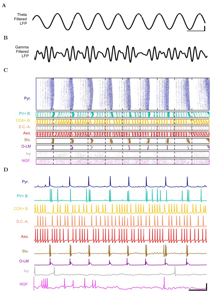
- The model contained 338,740 cells (311,500 pyramidal cells and 27,240 interneurons), 454,700 artificial stimulating afferents, and 5.19 billion synapses; it spontaneously produced stable theta at 7.8 Hz and gamma oscillations (25–80 Hz), with gamma amplitude phase-locked to the theta trough.
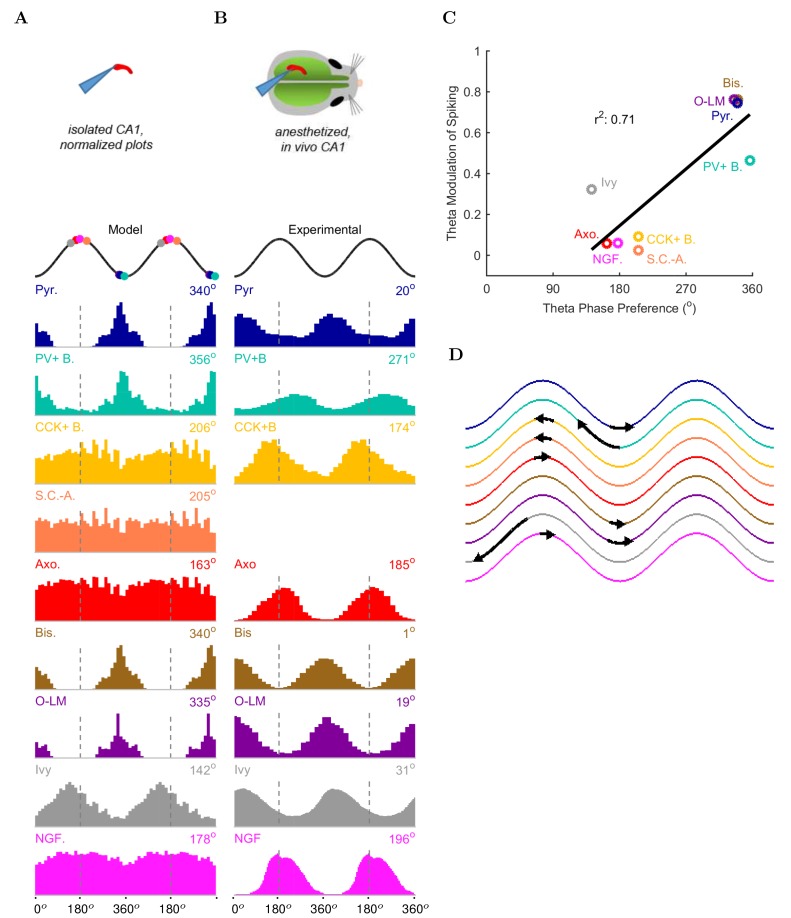
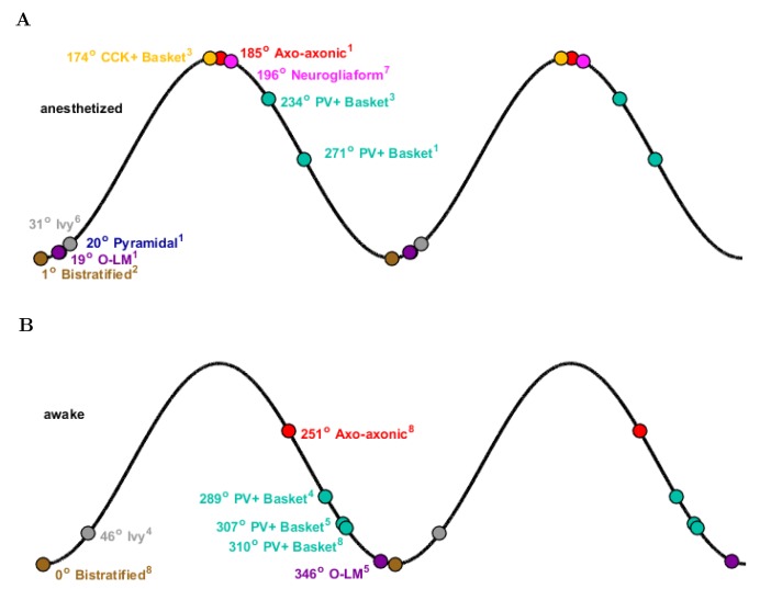
- Distinct interneuron types showed phase-preferential firing: PV+ basket, bistratified, and O-LM cells fired near the theta trough, whereas ivy, neurogliaform, CCK+ basket, and axo-axonic cells fired least around the trough; 71% (5/7) of interneuron types with experimental data matched anesthetized in vivo phase maxima.
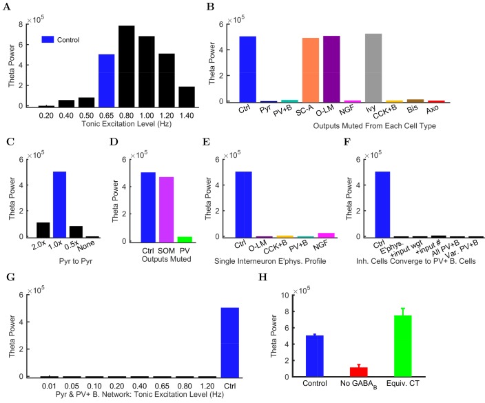
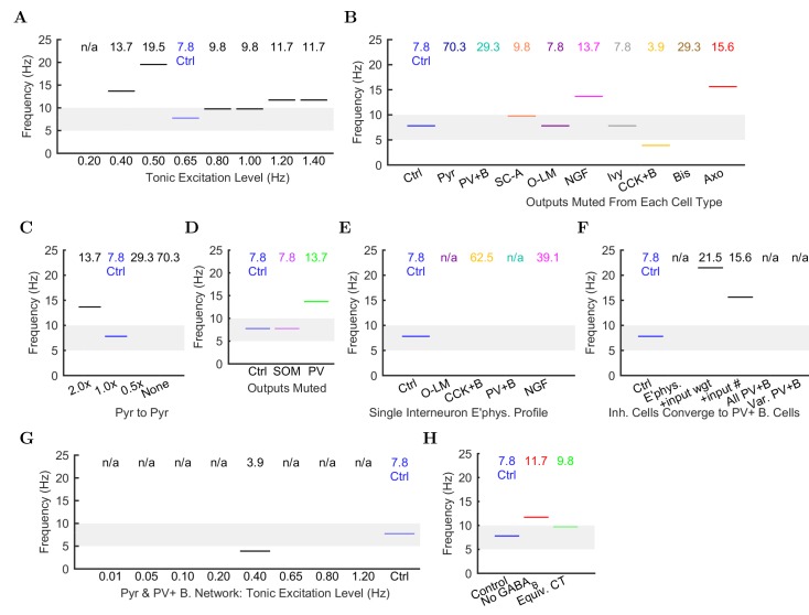
- Muting pyramidal cell output or CA1 pyramidal-to-pyramidal connections collapsed theta; muting PV-family, CCK+ basket, or neurogliaform cell output strongly reduced theta, while muting O-LM, ivy, or SC-A cells had no effect. Partial PV+ muting disrupted theta more than partial SOM+ muting.
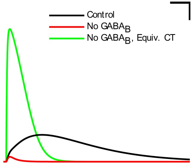
- Reducing interneuron diversity abolished theta: giving all interneurons one electrophysiological profile, or morphing them toward PV+ basket cells, did not restore theta. Removing the GABAB component of neurogliaform synapses reduced theta power, but replacing it with a scaled-up fast GABAA conductance with equivalent charge transfer restored theta.
Methods
- The CA1 network was implemented in parallel NEURON 7.4 with one multicompartmental pyramidal cell type and eight interneuron types; connectivity and cell numbers were taken from Bezaire and Soltesz (2013), and simulations used fixed time steps of 0.01–0.025 ms for 2000 or 4000 ms on supercomputers.
- CA3 and entorhinal afferents were modeled as independent Poisson spike trains; control theta emerged at a mean afferent firing rate of 0.65 Hz, and analyses included spike density functions, Welch periodograms, spectrograms, an LFP analog, Rayleigh tests for phase modulation, and ANOVA for GABAB-related simulations.
- Perturbation experiments muted each cell type’s output, altered pyramidal-to-pyramidal connection numbers, reduced interneuron diversity, and manipulated neurogliaform GABAB/GABAA signaling.
Limitations
- Stated: about 30% of known CA1 interneurons were omitted due to paucity of quantitative data, likely making inhibition weaker than biological; pyramidal cells fired more than in vivo, and although scaled-up inhibition produced only 1% active pyramidal cells firing at 1.8 Hz, it was not used because the source of the additional inhibition was unidentified.
- Stated: the model did not include neuromodulators, gap junctions, short-term plasticity, glial dynamics, pyramidal cell diversity, or cell-to-cell variability; the emergent theta likely resembled the atropine-resistant form, some single-cell electrophysiology came from mouse while the network was rat, and no isolated-CA1 data were available for interneuron phase preferences, so comparisons used anesthetized in vivo data.
- Evident: theta appeared only within particular afferent excitation levels (around 0.65 Hz; lower or higher levels disrupted it), gamma was not examined further, and the authors note they could not rule out a hypothetical theta regime somewhere in the low-diversity parameter space.
Model-written summary. Check it against the paper before relying on it.
Integrity signals
Registry
Cites
Statistics
Figures
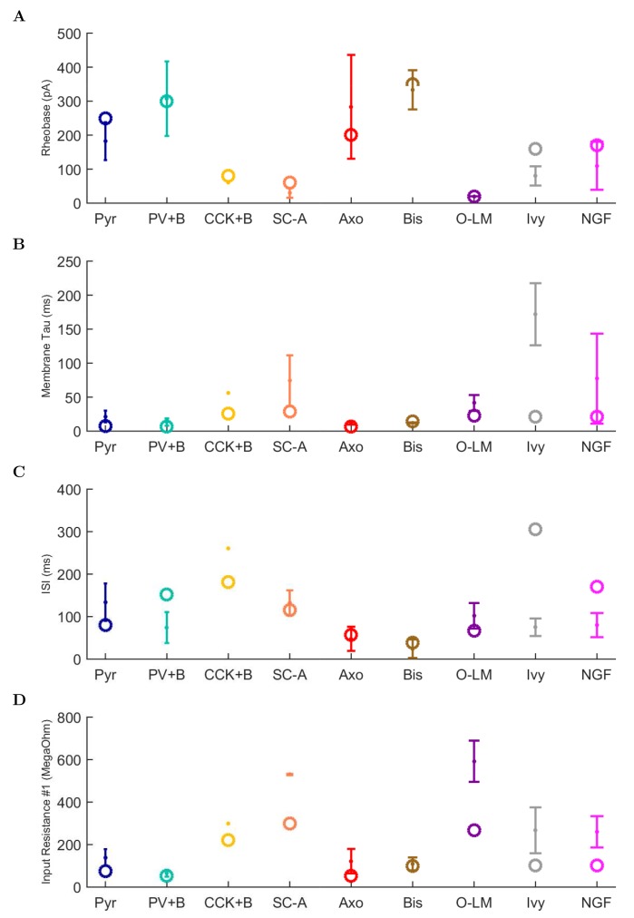
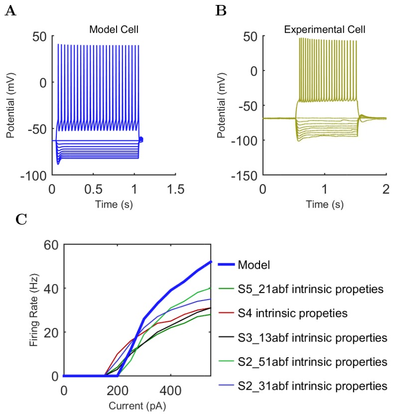
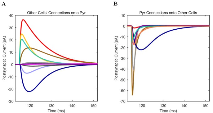
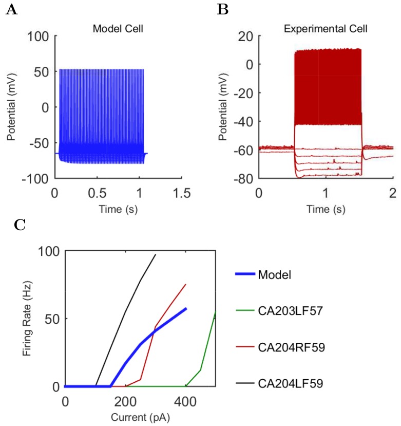
Verification
Claims the paper makes
53 Not checked yet · 46 Own result · 29 Own interpretation · 9 Own method · 6 No basis given · 1 Sources not found
None of the sources cited for this claim have been checked yet.
In the paper
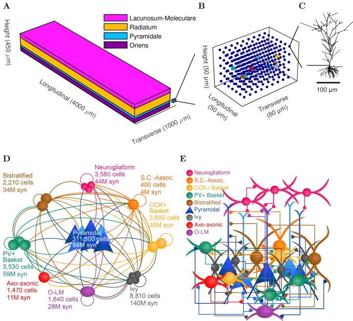
“The model network contained 338,740 cells (similar to the biological CA1 in rats, including 311,500 pyramidal cells and 27,240 interneurons) (Figure 1D–E and Figure 1—figure supplement 1).”
§ Interneuronal mechanisms of hippocampal theta oscillations in a full-scale model of the rodent CA1 circuit > Results > Development of a data-driven, full-scale model of the isolated CA1
plain- Asserted: passes — The authors put it forward as true.
- Checkable: passes — It can be checked against evidence.
- Load-bearing: passes — The paper’s conclusions depend on it.
- Based: passes — The paper gives a reason why it holds.
A result the paper reports from its own data — it cites no other source for it, so there is none to check. The quote shows it is in the paper.
In the paper
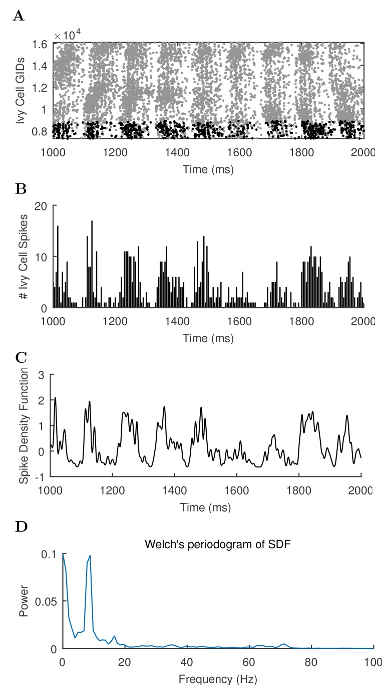
“We varied the magnitude of arrhythmic, tonic excitation to the network (by systematically changing the mean spiking frequency of the artificial stimulating cells, see above) and identified excitation levels where the network developed a stable, spontaneous theta rhythm (5–10 Hz; Figure 3 and 4; Figure 3—source data 1–3 and Figure 4—source data 1–2).”
§ Interneuronal mechanisms of hippocampal theta oscillations in a full-scale model of the rodent CA1 circuit > Results > Emergence of spontaneous theta and gamma oscillations in the full-scale model in the absence of rhythmic external inputs
plaindirect- Asserted: passes — The authors put it forward as true.
- Checkable: passes — It can be checked against evidence.
- Load-bearing: passes — The paper’s conclusions depend on it.
- Based: passes — The paper gives a reason why it holds.
The paper states this without a source or data behind it here, so there is nothing to check it against. The quote shows it is in the paper.
In the paper
“The afferent divergence and convergence onto the cells were also anatomically patterned, maintaining the topographical arrangement seen experimentally (Hongo et al., 2015), for a total of 5.19 billion synaptic connections in the model network.”
§ Interneuronal mechanisms of hippocampal theta oscillations in a full-scale model of the rodent CA1 circuit > Results > Development of a data-driven, full-scale model of the isolated CA1
plain- Asserted: passes — The authors put it forward as true.
- Checkable: passes — It can be checked against evidence.
- Load-bearing: passes — The paper’s conclusions depend on it.
- Based: passes — The paper gives a reason why it holds.
A result the paper reports from its own data — it cites no other source for it, so there is none to check. The quote shows it is in the paper.
In the paper
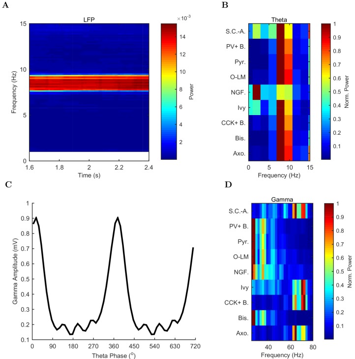
“The theta oscillation was stable, maintaining a steady power level throughout the duration of the oscillation (Figure 4A).”
§ Interneuronal mechanisms of hippocampal theta oscillations in a full-scale model of the rodent CA1 circuit > Results > Emergence of spontaneous theta and gamma oscillations in the full-scale model in the absence of rhythmic external inputs
plain- Asserted: passes — The authors put it forward as true.
- Checkable: passes — It can be checked against evidence.
- Load-bearing: unclear — It is unclear whether the paper’s conclusions depend on it.
- Based: passes — The paper gives a reason why it holds.
None of the sources cited for this claim have been checked yet.
In the paper
“In addition to theta rhythm, the model network displayed gamma oscillations (25–80 Hz; Figures 3B and 4D), as expected based on in vivo data (Soltesz and Deschênes, 1993; Tort et al., 2009; Colgin and Moser, 2010) and in vitro slice data showing 65–75 Hz gamma oscillations arising in response to theta rhythmic network stimulation (Butler et al., 2016).”
§ Interneuronal mechanisms of hippocampal theta oscillations in a full-scale model of the rodent CA1 circuit > Results > Emergence of spontaneous theta and gamma oscillations in the full-scale model in the absence of rhythmic external inputs
What the sources say
- Not checked yetcites Soltesz and Deschênes, 1993
- Not checked yetcites Tort et al., 2009 source
- Not checked yetcites Colgin and Moser, 2010
plain- Asserted: passes — The authors put it forward as true.
- Checkable: passes — It can be checked against evidence.
- Load-bearing: passes — The paper’s conclusions depend on it.
- Based: passes — The paper gives a reason why it holds.
A result the paper reports from its own data — it cites no other source for it, so there is none to check. The quote shows it is in the paper.
In the paper
“In all of these measures of network activity, theta was apparent within one theta period of the simulation start.”
§ Interneuronal mechanisms of hippocampal theta oscillations in a full-scale model of the rodent CA1 circuit > Results > Emergence of spontaneous theta and gamma oscillations in the full-scale model in the absence of rhythmic external inputs
plain- Asserted: passes — The authors put it forward as true.
- Checkable: passes — It can be checked against evidence.
- Load-bearing: unclear — It is unclear whether the paper’s conclusions depend on it.
- Based: passes — The paper gives a reason why it holds.
A result the paper reports from its own data — it cites no other source for it, so there is none to check. The quote shows it is in the paper.
In the paper
“The highest amplitude of the gamma oscillations in the model was observed at the theta trough (0°/360°) in the pyramidal layer LFP analog (Figure 4C).”
§ Interneuronal mechanisms of hippocampal theta oscillations in a full-scale model of the rodent CA1 circuit > Results > Emergence of spontaneous theta and gamma oscillations in the full-scale model in the absence of rhythmic external inputs
plaincorrelational- Asserted: passes — The authors put it forward as true.
- Checkable: passes — It can be checked against evidence.
- Load-bearing: unclear — It is unclear whether the paper’s conclusions depend on it.
- Based: passes — The paper gives a reason why it holds.
None of the sources cited for this claim have been checked yet.
In the paper
“The amplitude envelope of the gamma oscillation was phase-locked to the theta rhythm (Figures 3A,B and 4C), as it is in the biological CA1, representing cross-frequency coupling (Soltesz and Deschênes, 1993; Bragin et al., 1995; Buzsáki et al., 2003; Jensen and Colgin, 2007; Belluscio et al., 2012).”
§ Interneuronal mechanisms of hippocampal theta oscillations in a full-scale model of the rodent CA1 circuit > Results > Emergence of spontaneous theta and gamma oscillations in the full-scale model in the absence of rhythmic external inputs
What the sources say
plaincorrelational- Asserted: passes — The authors put it forward as true.
- Checkable: passes — It can be checked against evidence.
- Load-bearing: unclear — It is unclear whether the paper’s conclusions depend on it.
- Based: passes — The paper gives a reason why it holds.
A result the paper reports from its own data — it cites no other source for it, so there is none to check. The quote shows it is in the paper.
In the paper
“The pyramidal cell spikes (Figures 3C and D) exhibited peak power around the theta frequency of 7.8 Hz (Figure 4 and Table 7).”
§ Interneuronal mechanisms of hippocampal theta oscillations in a full-scale model of the rodent CA1 circuit > Results > Emergence of spontaneous theta and gamma oscillations in the full-scale model in the absence of rhythmic external inputs
plaincorrelational- Asserted: passes — The authors put it forward as true.
- Checkable: passes — It can be checked against evidence.
- Load-bearing: passes — The paper’s conclusions depend on it.
- Based: passes — The paper gives a reason why it holds.
None of the sources cited for this claim have been checked yet.
In the paper
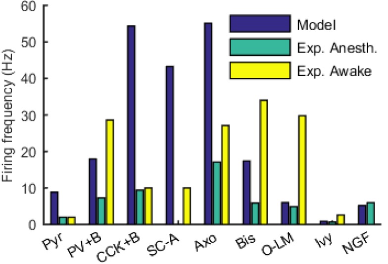
“Indeed, the pyramidal cells in our model described above (Figures 3 and 4) tended to fire more than they typically do during theta oscillations in vivo (e.g., [Soltesz and Deschênes, 1993; Robbe et al., 2006]).”
§ Interneuronal mechanisms of hippocampal theta oscillations in a full-scale model of the rodent CA1 circuit > Results > Emergence of spontaneous theta and gamma oscillations in the full-scale model in the absence of rhythmic external inputs
What the sources say
- Not checked yetcites Soltesz and Deschênes, 1993
- Not checked yetcites Robbe et al., 2006 source
hedgedcorrelational- Asserted: passes — The authors put it forward as true.
- Checkable: passes — It can be checked against evidence.
- Load-bearing: passes — The paper’s conclusions depend on it.
- Based: passes — The paper gives a reason why it holds.
- It may state two separate claims as one. 23
- Probably not a substantial claim. 37
None of the sources cited for this claim have been checked yet.
In the paper
“In simulations with the model containing this rationally scaled up inhibition, only 1% of the pyramidal cells were active, and they fired at a low rate of 1.8 Hz (data not shown), closely resembling the in vivo condition (Soltesz and Deschênes, 1993; Robbe et al., 2006).”
§ Interneuronal mechanisms of hippocampal theta oscillations in a full-scale model of the rodent CA1 circuit > Results > Emergence of spontaneous theta and gamma oscillations in the full-scale model in the absence of rhythmic external inputs
What the sources say
- Not checked yetcites Soltesz and Deschênes, 1993
- Not checked yetcites Robbe et al., 2006 source
plaindirect- Asserted: passes — The authors put it forward as true.
- Checkable: passes — It can be checked against evidence.
- Load-bearing: passes — The paper’s conclusions depend on it.
- Based: passes — The paper gives a reason why it holds.
It may state two separate claims as one.
A result the paper reports from its own data — it cites no other source for it, so there is none to check. The quote shows it is in the paper.
In the paper
“there was a correlation between the phase preference and the strength of modulation (Figure 5C; see Materials and methods), with the cells discharging around the trough all showing strong modulation of firing.”
§ Interneuronal mechanisms of hippocampal theta oscillations in a full-scale model of the rodent CA1 circuit > Results > Mechanism of theta generation and phase-preferential firing of interneurons in the full-scale model of the isolated CA1
plaincorrelational- Asserted: passes — The authors put it forward as true.
- Checkable: passes — It can be checked against evidence.
- Load-bearing: unclear — It is unclear whether the paper’s conclusions depend on it.
- Based: passes — The paper gives a reason why it holds.
It may state two separate claims as one.
A result the paper reports from its own data — it cites no other source for it, so there is none to check. The quote shows it is in the paper.
In the paper
“Theta phase preference and theta modulation level were correlated; better modulated cell types spiked closer to the LFP analog trough near the phase preference of pyramidal cells.”
§ Interneuronal mechanisms of hippocampal theta oscillations in a full-scale model of the rodent CA1 circuit > Results > Mechanism of theta generation and phase-preferential firing of interneurons in the full-scale model of the isolated CA1
plaincorrelational- Asserted: passes — The authors put it forward as true.
- Checkable: passes — It can be checked against evidence.
- Load-bearing: passes — The paper’s conclusions depend on it.
- Based: passes — The paper gives a reason why it holds.
It may state two separate claims as one.
- Rests on an assumption: The experimental phase preferences from anesthetized rats are comparable to the model's conditions.
In the paper
“when the excitation level increased beyond 0.80 Hz, theta power also started to drop significantly as the oscillation frequency rose out of theta range (Figure 6 and Figure 6—figure supplement 1; Figure 6—source data 1–2), evolving into a beta oscillation (Engel and Fries, 2010).”
§ Interneuronal mechanisms of hippocampal theta oscillations in a full-scale model of the rodent CA1 circuit > Results > Perturbation experiments indicate a key role for interneuronal diversity in the emergence of spontaneous theta
What the sources say
- Not checked yetcites Engel and Fries, 2010 source
plaindirect- Asserted: passes — The authors put it forward as true.
- Checkable: passes — It can be checked against evidence.
- Load-bearing: passes — The paper’s conclusions depend on it.
- Based: passes — The paper gives a reason why it holds.
It may state two separate claims as one.
A result the paper reports from its own data — it cites no other source for it, so there is none to check. The quote shows it is in the paper.
In the paper
“Cell type-specific perturbations of the network showed that each interneuronal type contributed uniquely to the spontaneous theta oscillation, and that the presence of diverse inhibitory dynamics was a necessary condition for sustained theta oscillations.”
§ Interneuronal mechanisms of hippocampal theta oscillations in a full-scale model of the rodent CA1 circuit > Discussion > Emergence of theta oscillations from a biological data-driven, full-scale model of the CA1 network
plaindirect- Asserted: passes — The authors put it forward as true.
- Checkable: passes — It can be checked against evidence.
- Load-bearing: passes — The paper’s conclusions depend on it.
- Based: passes — The paper gives a reason why it holds.
It may state two separate claims as one.
The paper states this without a source or data behind it here, so there is nothing to check it against. The quote shows it is in the paper.
In the paper
“As none of the model neurons in our model CA1 network are spontaneously active”
§ Interneuronal mechanisms of hippocampal theta oscillations in a full-scale model of the rodent CA1 circuit > Materials and methods > Stimulation
plain- Asserted: passes — The authors put it forward as true.
- Checkable: passes — It can be checked against evidence.
- Load-bearing: passes — The paper’s conclusions depend on it.
- Based: fails — The paper may give no reason why it holds.
Probably not a substantial claim. The paper may give no reason why it holds.
None of the sources cited for this claim have been checked yet.
In the paper
“In rodents, hippocampal theta is a 5–10 Hz oscillation in the local field potential (LFP) and neuronal firing probabilities (Soltesz and Deschênes, 1993; Lee et al., 1994; Ylinen et al., 1995; Klausberger and Somogyi, 2008; Varga et al., 2012, 2014), occurring during locomotion and in REM sleep (Buzsáki, 2002).”
§ Interneuronal mechanisms of hippocampal theta oscillations in a full-scale model of the rodent CA1 circuit > Introduction
What the sources say
plaincorrelational- Asserted: passes — The authors put it forward as true.
- Checkable: passes — It can be checked against evidence.
- Load-bearing: fails — The paper’s conclusions may not depend on it.
- Based: passes — The paper gives a reason why it holds.
Probably not a substantial claim. The paper’s conclusions may not depend on it. It may state two separate claims as one.
The paper states this without a source or data behind it here, so there is nothing to check it against. The quote shows it is in the paper.
In the paper
“In principle, such full-scale models of mammalian circuits comprising hundreds of thousands of neurons of distinct types advantageously avoid the connectivity scaling tradeoff that besets reduced-scale models”
§ Interneuronal mechanisms of hippocampal theta oscillations in a full-scale model of the rodent CA1 circuit > Introduction
hedgeddirect- Asserted: passes — The authors put it forward as true.
- Checkable: passes — It can be checked against evidence.
- Load-bearing: passes — The paper’s conclusions depend on it.
- Based: passes — The paper gives a reason why it holds.
Probably not a substantial claim.
In the paper
“Cell type-specific connectivity data, including cell numbers (Figure 1D) and convergence and divergence values (Figure 1E; Figure 1—figure supplement 1 and Table 1) were taken without alteration from our previously published, in-depth, quantitative assessment of the CA1 circuit (Bezaire and Soltesz, 2013).”
§ Interneuronal mechanisms of hippocampal theta oscillations in a full-scale model of the rodent CA1 circuit > Results > Development of a data-driven, full-scale model of the isolated CA1
What the sources say
- Not checked yetcites Bezaire and Soltesz, 2013 source
plain- Asserted: passes — The authors put it forward as true.
- Checkable: passes — It can be checked against evidence.
- Load-bearing: passes — The paper’s conclusions depend on it.
- Based: passes — The paper gives a reason why it holds.
Probably not a substantial claim.
In the paper
“The remaining 30% of the interneurons were not included in the model due to paucity of quantitative data (Bezaire and Soltesz, 2013).”
§ Interneuronal mechanisms of hippocampal theta oscillations in a full-scale model of the rodent CA1 circuit > Results > Development of a data-driven, full-scale model of the isolated CA1
What the sources say
- Not checked yetcites Bezaire and Soltesz, 2013 source
plaindirect- Asserted: passes — The authors put it forward as true.
- Checkable: passes — It can be checked against evidence.
- Load-bearing: fails — The paper’s conclusions may not depend on it.
- Based: passes — The paper gives a reason why it holds.
Probably not a substantial claim. The paper’s conclusions may not depend on it.
In the paper
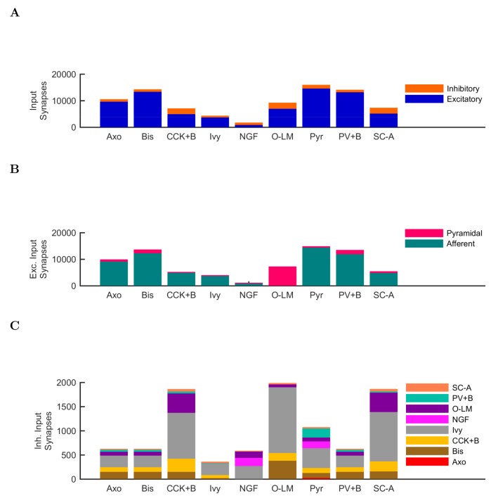
“note that PV+ cells receive a high number of excitatory inputs on their dendrites compared to other interneuron classes (Gulyás et al., 1999).”
§ Interneuronal mechanisms of hippocampal theta oscillations in a full-scale model of the rodent CA1 circuit > Results > Mechanism of theta generation and phase-preferential firing of interneurons in the full-scale model of the isolated CA1
What the sources say
- Not checked yetcites Gulyás et al., 1999 source
plaincorrelational- Asserted: passes — The authors put it forward as true.
- Checkable: passes — It can be checked against evidence.
- Load-bearing: fails — The paper’s conclusions may not depend on it.
- Based: passes — The paper gives a reason why it holds.
Probably not a substantial claim. The paper’s conclusions may not depend on it.
None of the sources cited for this claim have been checked yet.
In the paper
“As mentioned above, distinct interneuronal types, defined based on their selective axonal innervation patterns of the postsynaptic domains of pyramidal cells, exhibit characteristic, cell-type-specific preferred phases of firing during theta oscillations in vivo (Klausberger et al., 2003; 2004, 2005; Ferraguti et al., 2005; Jinno et al., 2007; Fuentealba et al., 2008; Varga et al., 2012; Lapray et”
§ Interneuronal mechanisms of hippocampal theta oscillations in a full-scale model of the rodent CA1 circuit > Results > Mechanism of theta generation and phase-preferential firing of interneurons in the full-scale model of the isolated CA1
What the sources say
plaincorrelational- Asserted: passes — The authors put it forward as true.
- Checkable: passes — It can be checked against evidence.
- Load-bearing: passes — The paper’s conclusions depend on it.
- Based: passes — The paper gives a reason why it holds.
Probably not a substantial claim.
In the paper
“As expected, the numerically dominant pyramidal cells, whose intracellular membrane potential oscillations to a large extent generate and underlie the extracellular LFP signal during theta oscillations (Buzsáki et al., 2012), preferentially discharged around the trough 0o/360o of the LFP analog theta rhythm (Figure 5A).”
§ Interneuronal mechanisms of hippocampal theta oscillations in a full-scale model of the rodent CA1 circuit > Results > Mechanism of theta generation and phase-preferential firing of interneurons in the full-scale model of the isolated CA1
What the sources say
- Not checked yetcites Buzsáki et al., 2012 source
plaindirect- Asserted: passes — The authors put it forward as true.
- Checkable: passes — It can be checked against evidence.
- Load-bearing: fails — The paper’s conclusions may not depend on it.
- Based: passes — The paper gives a reason why it holds.
Probably not a substantial claim. The paper’s conclusions may not depend on it.
In the paper
“key roles for inter-pyramidal cell excitatory synapses within CA1 have been suggested for sharp wave ripple oscillations as well (Maier et al., 2011).”
§ Interneuronal mechanisms of hippocampal theta oscillations in a full-scale model of the rodent CA1 circuit > Results > Perturbation experiments indicate a key role for interneuronal diversity in the emergence of spontaneous theta
What the sources say
- Not checked yetcites Maier et al., 2011 source
hedgedconditional- Asserted: passes — The authors put it forward as true.
- Checkable: passes — It can be checked against evidence.
- Load-bearing: fails — The paper’s conclusions may not depend on it.
- Based: passes — The paper gives a reason why it holds.
Probably not a substantial claim. The paper’s conclusions may not depend on it.
A conclusion the paper draws from its own results — it cites no other source for it, so there is none to check. The quote shows it is in the paper.
In the paper
“These data indicate that while synaptic-cellular organization of the CA1 circuit enables the intrinsic, within-CA1 generation of theta waves, the circuit is predisposed to exhibit theta oscillations only under particular excitatory input conditions.”
§ Interneuronal mechanisms of hippocampal theta oscillations in a full-scale model of the rodent CA1 circuit > Results > Perturbation experiments indicate a key role for interneuronal diversity in the emergence of spontaneous theta
hedgedconditional- Asserted: passes — The authors put it forward as true.
- Checkable: passes — It can be checked against evidence.
- Load-bearing: passes — The paper’s conclusions depend on it.
- Based: passes — The paper gives a reason why it holds.
It may state two separate claims as one.
None of the sources cited for this claim have been checked yet.
In the paper
“Since the diverse sources of inhibition from the various interneuronal types are believed to enable networks to achieve more complex behaviors, including oscillations (Soltesz, 2006; Rotstein et al., 2005; Kepecs and Fishell, 2014)”
§ Interneuronal mechanisms of hippocampal theta oscillations in a full-scale model of the rodent CA1 circuit > Results > Perturbation experiments indicate a key role for interneuronal diversity in the emergence of spontaneous theta
What the sources say
hedgedconditional- Asserted: passes — The authors put it forward as true.
- Checkable: passes — It can be checked against evidence.
- Load-bearing: passes — The paper’s conclusions depend on it.
- Based: passes — The paper gives a reason why it holds.
Probably not a substantial claim.
In the paper
“First, we studied the role of the recurrent collaterals of pyramidal cells, which contact mostly interneurons and, less frequently, other pyramidal cells (Bezaire and Soltesz, 2013).”
§ Interneuronal mechanisms of hippocampal theta oscillations in a full-scale model of the rodent CA1 circuit > Results > Perturbation experiments indicate a key role for interneuronal diversity in the emergence of spontaneous theta
What the sources say
- Not checked yetcites Bezaire and Soltesz, 2013 source
plain- Asserted: passes — The authors put it forward as true.
- Checkable: passes — It can be checked against evidence.
- Load-bearing: fails — The paper’s conclusions may not depend on it.
- Based: passes — The paper gives a reason why it holds.
Probably not a substantial claim. The paper’s conclusions may not depend on it.
None of the sources cited for this claim have been checked yet.
In the paper
“we focused on PV+ basket cells, which have been implicated in theta generation in vivo (Soltesz and Deschênes, 1993; Buzsáki, 2002; Stark et al., 2013; Hu et al., 2014)”
§ Interneuronal mechanisms of hippocampal theta oscillations in a full-scale model of the rodent CA1 circuit > Results > Perturbation experiments indicate a key role for interneuronal diversity in the emergence of spontaneous theta
What the sources say
plaincorrelational- Asserted: passes — The authors put it forward as true.
- Checkable: passes — It can be checked against evidence.
- Load-bearing: passes — The paper’s conclusions depend on it.
- Based: passes — The paper gives a reason why it holds.
Probably not a substantial claim.
A conclusion the paper draws from its own results — it cites no other source for it, so there is none to check. The quote shows it is in the paper.
In the paper
“These abilities may serve to maintain the stability and robustness of the theta oscillation mechanism as it operates in vivo in diverse behavioral states.”
§ Interneuronal mechanisms of hippocampal theta oscillations in a full-scale model of the rodent CA1 circuit > Discussion > Emergence of theta oscillations from a biological data-driven, full-scale model of the CA1 network
hedgedconditional- Asserted: passes — The authors put it forward as true.
- Checkable: fails — It may be too vague to check against evidence.
- Load-bearing: fails — The paper’s conclusions may not depend on it.
- Based: fails — The paper may give no reason why it holds.
Probably not a substantial claim. It may be too vague to check against evidence. The paper’s conclusions may not depend on it. The paper may give no reason why it holds.
A conclusion the paper draws from its own results — it cites no other source for it, so there is none to check. The quote shows it is in the paper.
In the paper
“Therefore, muting the neurogliaform cells strongly disrupted the theta oscillations not because the theta oscillations required the slow kinetics of GABAB IPSPs specifically, but because the slow kinetics enabled a large total charge transfer.”
§ Interneuronal mechanisms of hippocampal theta oscillations in a full-scale model of the rodent CA1 circuit > Results > Neurogliaform cell signaling and theta generation in the isolated CA1 model
plaindirect- Asserted: passes — The authors put it forward as true.
- Checkable: passes — It can be checked against evidence.
- Load-bearing: passes — The paper’s conclusions depend on it.
- Based: passes — The paper gives a reason why it holds.
It may state two separate claims as one.
In the paper
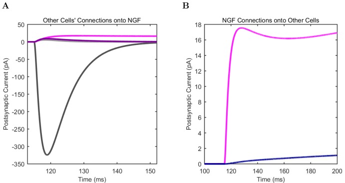
“These two model interneuron groups mainly differed in that the neurogliaform cells evoked mixed GABAA,B postsynaptic events (Price et al., 2005), whereas the model ivy cells only triggered GABAA IPSPs (in agreement with a lack of evidence for ivy cell-evoked GABAB IPSPs).”
§ Interneuronal mechanisms of hippocampal theta oscillations in a full-scale model of the rodent CA1 circuit > Results > Neurogliaform cell signaling and theta generation in the isolated CA1 model
What the sources say
- Not checked yetcites Price et al., 2005 source
plaindirect- Asserted: passes — The authors put it forward as true.
- Checkable: passes — It can be checked against evidence.
- Load-bearing: passes — The paper’s conclusions depend on it.
- Based: passes — The paper gives a reason why it holds.
It may state two separate claims as one.
In the paper
“Therefore, although PV basket cells appear to be important for theta-generation both in the biological and the model CA1 network, endowing all interneurons with PV basket cell-like properties does not lead to a network configuration conducive to theta oscillations (Hendrickson et al., 2015).”
§ Interneuronal mechanisms of hippocampal theta oscillations in a full-scale model of the rodent CA1 circuit > Results > Perturbation experiments indicate a key role for interneuronal diversity in the emergence of spontaneous theta
What the sources say
- Not checked yetcites Hendrickson et al., 2015 source
hedgeddirect- Asserted: passes — The authors put it forward as true.
- Checkable: passes — It can be checked against evidence.
- Load-bearing: passes — The paper’s conclusions depend on it.
- Based: passes — The paper gives a reason why it holds.
It may state two separate claims as one.
A conclusion the paper draws from its own results — it cites no other source for it, so there is none to check. The quote shows it is in the paper.
In the paper
“these model results generally suggest that the presence of diverse interneuronal types and the intrinsic circuitry of the CA1 network are sufficient and necessary to enable the isolated CA1 to oscillate at spontaneous theta rhythms while supporting distinct phase preferences of each class of hippocampal neuron.”
§ Interneuronal mechanisms of hippocampal theta oscillations in a full-scale model of the rodent CA1 circuit > Discussion > Emergence of theta oscillations from a biological data-driven, full-scale model of the CA1 network
hedgeddirect- Asserted: passes — The authors put it forward as true.
- Checkable: passes — It can be checked against evidence.
- Load-bearing: passes — The paper’s conclusions depend on it.
- Based: passes — The paper gives a reason why it holds.
It may state two separate claims as one.
None of the sources cited for this claim have been checked yet.
In the paper
“About 250,000 principal cells from ipsilateral ECIII synapse onto the CA1 region (Andersen et al., 2006), and approximately 2% of these cells are active per theta cycle at a low firing rate (Csicsvari et al., 1999; Mizuseki et al., 2009). Therefore, ECIII cells could provide 5000 input spikes to ipsilateral CA1 (Equation 3).”
§ Interneuronal mechanisms of hippocampal theta oscillations in a full-scale model of the rodent CA1 circuit > Discussion > Emergence of theta oscillations from a biological data-driven, full-scale model of the CA1 network
What the sources say
hedged- Asserted: passes — The authors put it forward as true.
- Checkable: passes — It can be checked against evidence.
- Load-bearing: passes — The paper’s conclusions depend on it.
- Based: passes — The paper gives a reason why it holds.
It may state two separate claims as one.
A conclusion the paper draws from its own results — it cites no other source for it, so there is none to check. The quote shows it is in the paper.
In the paper
“Such a large conductance is not biologically realistic, indicating that the key role for GABAB synapses may be to allow the large synaptic charge transfer via a temporal distribution.”
§ Interneuronal mechanisms of hippocampal theta oscillations in a full-scale model of the rodent CA1 circuit > Discussion > Emergence of theta oscillations from a biological data-driven, full-scale model of the CA1 network
hedgedconditional- Asserted: passes — The authors put it forward as true.
- Checkable: passes — It can be checked against evidence.
- Load-bearing: passes — The paper’s conclusions depend on it.
- Based: passes — The paper gives a reason why it holds.
It may state two separate claims as one.
A conclusion the paper draws from its own results — it cites no other source for it, so there is none to check. The quote shows it is in the paper.
In the paper
“Therefore, about 37,750 spikes per theta cycle arrive from ipsilateral CA3 and entorhinal cortex to the CA1 network in vivo, which is reassuringly close to the our modeling results indicating that robust theta emerged when the CA1 network model received approximately 37,900 afferent spikes per theta cycle.”
§ Interneuronal mechanisms of hippocampal theta oscillations in a full-scale model of the rodent CA1 circuit > Discussion > Emergence of theta oscillations from a biological data-driven, full-scale model of the CA1 network
plaincorrelational- Asserted: passes — The authors put it forward as true.
- Checkable: passes — It can be checked against evidence.
- Load-bearing: passes — The paper’s conclusions depend on it.
- Based: passes — The paper gives a reason why it holds.
It may state two separate claims as one.
None of the sources cited for this claim have been checked yet.
In the paper
“In turn, phase preferential firing may aid information processing tasks by providing order and allowing multiple channels of information to be processed in parallel (Jensen and Lisman, 2000; Hasselmo et al., 2002; Womelsdorf et al., 2007; Schomburg et al., 2014; Jeewajee et al., 2014; Maris et al., 2016).”
§ Interneuronal mechanisms of hippocampal theta oscillations in a full-scale model of the rodent CA1 circuit > Discussion > Emergence of theta oscillations from a biological data-driven, full-scale model of the CA1 network
What the sources say
hedgedconditional- Asserted: passes — The authors put it forward as true.
- Checkable: passes — It can be checked against evidence.
- Load-bearing: fails — The paper’s conclusions may not depend on it.
- Based: passes — The paper gives a reason why it holds.
Probably not a substantial claim. The paper’s conclusions may not depend on it. It may state two separate claims as one.
A conclusion the paper draws from its own results — it cites no other source for it, so there is none to check. The quote shows it is in the paper.
In the paper
“potentially indicating the primary importance of pyramidal cell inputs in driving these interneurons to fire during theta oscillations under all conditions”
§ Interneuronal mechanisms of hippocampal theta oscillations in a full-scale model of the rodent CA1 circuit > Discussion > Rationale for bases of comparison between modeling results with experimental data
hedgeddirect- Asserted: passes — The authors put it forward as true.
- Checkable: passes — It can be checked against evidence.
- Load-bearing: fails — The paper’s conclusions may not depend on it.
- Based: passes — The paper gives a reason why it holds.
Probably not a substantial claim. The paper’s conclusions may not depend on it.
None of the sources cited for this claim have been checked yet.
In the paper
“Indeed, the importance of GABAB receptors has also been indicated by a number of recent experimental studies, for example, in the modulation of theta and gamma oscillations (Kohl and Paulsen, 2010), setting of spike timing of neuron types during theta (Kohl and Paulsen, 2010), and playing a role in cortical oscillations and memory processes (Craig and McBain, 2014).”
§ Interneuronal mechanisms of hippocampal theta oscillations in a full-scale model of the rodent CA1 circuit > Discussion > Emergence of theta oscillations from a biological data-driven, full-scale model of the CA1 network
What the sources say
- Not checked yetcites Kohl and Paulsen, 2010
- Not checked yetcites Craig and McBain, 2014
hedgedcorrelational- Asserted: passes — The authors put it forward as true.
- Checkable: passes — It can be checked against evidence.
- Load-bearing: fails — The paper’s conclusions may not depend on it.
- Based: passes — The paper gives a reason why it holds.
Probably not a substantial claim. The paper’s conclusions may not depend on it. It may state two separate claims as one.
In the paper
“We previously estimated 204,700 pyramidal cells in ipsilateral CA3 (Bezaire and Soltesz, 2013), giving an estimated 32,750 spikes from ipsilateral CA3 per theta cycle (Equation 2).”
§ Interneuronal mechanisms of hippocampal theta oscillations in a full-scale model of the rodent CA1 circuit > Discussion > Emergence of theta oscillations from a biological data-driven, full-scale model of the CA1 network
What the sources say
- Not checked yetcites Bezaire and Soltesz, 2013 source
hedgeddirect- Asserted: passes — The authors put it forward as true.
- Checkable: passes — It can be checked against evidence.
- Load-bearing: passes — The paper’s conclusions depend on it.
- Based: passes — The paper gives a reason why it holds.
It may state two separate claims as one.
None of the sources cited for this claim have been checked yet.
In the paper
“The theta rhythm is thought to be important for organizing disparate memory tasks (Lisman and Idiart, 1995; Hasselmo et al., 2002; Hasselmo, 2005; Lisman and Jensen, 2013; Siegle and Wilson, 2014)”
§ Interneuronal mechanisms of hippocampal theta oscillations in a full-scale model of the rodent CA1 circuit > Discussion > Emergence of theta oscillations from a biological data-driven, full-scale model of the CA1 network
What the sources say
hedgedconditional- Asserted: passes — The authors put it forward as true.
- Checkable: passes — It can be checked against evidence.
- Load-bearing: fails — The paper’s conclusions may not depend on it.
- Based: passes — The paper gives a reason why it holds.
Probably not a substantial claim. The paper’s conclusions may not depend on it.
None of the sources cited for this claim have been checked yet.
In the paper
“a CA1 network which has evolved a predisposition to oscillate at theta and gamma frequencies may enable more efficient processing of the phasic input it receives in vivo (Akam and Kullmann, 2012; Fries, 2015).”
§ Interneuronal mechanisms of hippocampal theta oscillations in a full-scale model of the rodent CA1 circuit > Discussion > Emergence of theta oscillations from a biological data-driven, full-scale model of the CA1 network
What the sources say
hedgedconditional- Asserted: passes — The authors put it forward as true.
- Checkable: fails — It may be too vague to check against evidence.
- Load-bearing: fails — The paper’s conclusions may not depend on it.
- Based: passes — The paper gives a reason why it holds.
Probably not a substantial claim. It may be too vague to check against evidence. The paper’s conclusions may not depend on it.
A conclusion the paper draws from its own results — it cites no other source for it, so there is none to check. The quote shows it is in the paper.
In the paper
“In addition, the simulations unexpectedly revealed that interneuronal diversity itself may also be important in theta generation, since conversion of all interneurons into fast spiking PV+ basket cells did not result in a network that was conducive for the emergence of theta, in spite of the key role of the PV+ basket cells in hippocampal oscillations.”
§ Interneuronal mechanisms of hippocampal theta oscillations in a full-scale model of the rodent CA1 circuit > Discussion > Emergence of theta oscillations from a biological data-driven, full-scale model of the CA1 network
hedgedconditionalSingle case- Asserted: passes — The authors put it forward as true.
- Checkable: passes — It can be checked against evidence.
- Load-bearing: passes — The paper’s conclusions depend on it.
- Based: passes — The paper gives a reason why it holds.
It may state two separate claims as one.
- Rests on an assumption: The parameter space explored for low-diversity configurations is sufficient to conclude that interneuronal diversity is necessary for spontaneous theta oscillations.
In the paper
“The biological CA1 network receives most of its input from CA3 and entorhinal cortical layer III (ECIII), and it has been estimated that about 4% of CA3 pyramidal cells fire up to four spikes per theta wave (Gasparini and Magee, 2006).”
§ Interneuronal mechanisms of hippocampal theta oscillations in a full-scale model of the rodent CA1 circuit > Discussion > Emergence of theta oscillations from a biological data-driven, full-scale model of the CA1 network
What the sources say
- Not checked yetcites Gasparini and Magee, 2006
hedged- Asserted: passes — The authors put it forward as true.
- Checkable: passes — It can be checked against evidence.
- Load-bearing: passes — The paper’s conclusions depend on it.
- Based: passes — The paper gives a reason why it holds.
It may state two separate claims as one.
In the paper
“we have made freely available our custom software SimTracker (RRID:SCR_014735) that works with the model code to support each step of the modeling process”
§ Interneuronal mechanisms of hippocampal theta oscillations in a full-scale model of the rodent CA1 circuit > Discussion > An accessible approach to modeling that balances detail, scale, flexibility and performance
What the sources say
- Not checked yetcites Bezaire et al., 2016a
plaindirect- Asserted: passes — The authors put it forward as true.
- Checkable: passes — It can be checked against evidence.
- Load-bearing: fails — The paper’s conclusions may not depend on it.
- Based: passes — The paper gives a reason why it holds.
Probably not a substantial claim. The paper’s conclusions may not depend on it. It may state two separate claims as one.
A conclusion the paper draws from its own results — it cites no other source for it, so there is none to check. The quote shows it is in the paper.
In the paper
“it also plausible that both forms of theta benefit from occurring in a network that is predisposed to oscillate at the theta frequency, as the model network results suggested”
§ Interneuronal mechanisms of hippocampal theta oscillations in a full-scale model of the rodent CA1 circuit > Discussion > Rationale for bases of comparison between modeling results with experimental data
hedgedconditional- Asserted: passes — The authors put it forward as true.
- Checkable: passes — It can be checked against evidence.
- Load-bearing: fails — The paper’s conclusions may not depend on it.
- Based: passes — The paper gives a reason why it holds.
Probably not a substantial claim. The paper’s conclusions may not depend on it.
What the paper did — it cites no source for this, so there is none to check. The quote shows it is in the paper.
In the paper
“the model can be run on the Neuroscience Gateway, an online portal for accessing supercomputers that does not require technical knowledge of supercomputing”
§ Interneuronal mechanisms of hippocampal theta oscillations in a full-scale model of the rodent CA1 circuit > Discussion > An accessible approach to modeling that balances detail, scale, flexibility and performance
plain- Asserted: passes — The authors put it forward as true.
- Checkable: passes — It can be checked against evidence.
- Load-bearing: passes — The paper’s conclusions depend on it.
- Based: passes — The paper gives a reason why it holds.
Probably not a substantial claim.
In the paper
“the latter requires intact, rhythmic cholinergic inputs”
§ Interneuronal mechanisms of hippocampal theta oscillations in a full-scale model of the rodent CA1 circuit > Discussion > Rationale for bases of comparison between modeling results with experimental data
What the sources say
- Not checked yetcites Kramis et al., 1975 source
plaindirect- Asserted: passes — The authors put it forward as true.
- Checkable: passes — It can be checked against evidence.
- Load-bearing: passes — The paper’s conclusions depend on it.
- Based: passes — The paper gives a reason why it holds.
Probably not a substantial claim.
A conclusion the paper draws from its own results — it cites no other source for it, so there is none to check. The quote shows it is in the paper.
In the paper
“Such models are not subject to the connectivity scaling tradeoff wherein smaller networks have unrealistically low levels of input or unrealistically high connectivity between cells”
§ Interneuronal mechanisms of hippocampal theta oscillations in a full-scale model of the rodent CA1 circuit > Discussion > Conclusion and outlook
plain- Asserted: passes — The authors put it forward as true.
- Checkable: passes — It can be checked against evidence.
- Load-bearing: passes — The paper’s conclusions depend on it.
- Based: fails — The paper may give no reason why it holds.
Probably not a substantial claim. The paper may give no reason why it holds.
A conclusion the paper draws from its own results — it cites no other source for it, so there is none to check. The quote shows it is in the paper.
In the paper
“Our previous model has demonstrated how the resource intensive process of designing a detailed, large-scale model is offset by its potential usage in numerous ways by a multitude of groups”
§ Interneuronal mechanisms of hippocampal theta oscillations in a full-scale model of the rodent CA1 circuit > Discussion > An accessible approach to modeling that balances detail, scale, flexibility and performance
boosteddirect- Asserted: passes — The authors put it forward as true.
- Checkable: fails — It may be too vague to check against evidence.
- Load-bearing: fails — The paper’s conclusions may not depend on it.
- Based: passes — The paper gives a reason why it holds.
Probably not a substantial claim. It may be too vague to check against evidence. The paper’s conclusions may not depend on it.
A conclusion the paper draws from its own results — it cites no other source for it, so there is none to check. The quote shows it is in the paper.
In the paper
“It provides specific testable predictions that enable focused design of future experiments”
§ Interneuronal mechanisms of hippocampal theta oscillations in a full-scale model of the rodent CA1 circuit > Discussion > Conclusion and outlook
plaindirect- Asserted: passes — The authors put it forward as true.
- Checkable: passes — It can be checked against evidence.
- Load-bearing: passes — The paper’s conclusions depend on it.
- Based: passes — The paper gives a reason why it holds.
Probably not a substantial claim.
None of the sources cited for this claim have been checked yet.
In the paper
“Previously, we built a dentate gyrus model to study epileptic network dynamics (Santhakumar et al., 2005; Morgan and Soltesz, 2008) that was then used by several groups to study disparate topics including epilepsy, network mechanisms of inhibition and excitability, simulation optimization, and modeling software”
§ Interneuronal mechanisms of hippocampal theta oscillations in a full-scale model of the rodent CA1 circuit > Discussion > An accessible approach to modeling that balances detail, scale, flexibility and performance
What the sources say
plaindirect- Asserted: passes — The authors put it forward as true.
- Checkable: passes — It can be checked against evidence.
- Load-bearing: fails — The paper’s conclusions may not depend on it.
- Based: passes — The paper gives a reason why it holds.
Probably not a substantial claim. The paper’s conclusions may not depend on it.
None of the sources cited for this claim have been checked yet.
In the paper
“there is an increasing recognition in neurobiology that we must compile our collective experimental observations of the brain into something more cohesive and synergistic than what is being conveyed in individual research articles”
§ Interneuronal mechanisms of hippocampal theta oscillations in a full-scale model of the rodent CA1 circuit > Discussion > Conclusion and outlook
What the sources say
plain- Asserted: passes — The authors put it forward as true.
- Checkable: fails — It may be too vague to check against evidence.
- Load-bearing: fails — The paper’s conclusions may not depend on it.
- Based: passes — The paper gives a reason why it holds.
Probably not a substantial claim. It may be too vague to check against evidence. The paper’s conclusions may not depend on it.
In the paper
“the former is typically associated with walking and may not be dependent on neuromodulatory inputs”
§ Interneuronal mechanisms of hippocampal theta oscillations in a full-scale model of the rodent CA1 circuit > Discussion > Rationale for bases of comparison between modeling results with experimental data
What the sources say
- Not checked yetcites Kramis et al., 1975 source
hedgedcorrelational- Asserted: passes — The authors put it forward as true.
- Checkable: passes — It can be checked against evidence.
- Load-bearing: passes — The paper’s conclusions depend on it.
- Based: passes — The paper gives a reason why it holds.
Probably not a substantial claim. It may state two separate claims as one.
What the paper did — it cites no source for this, so there is none to check. The quote shows it is in the paper.
In the paper
“The model is public, well documented, and also well characterized in experimentally relevant terms”
§ Interneuronal mechanisms of hippocampal theta oscillations in a full-scale model of the rodent CA1 circuit > Discussion > An accessible approach to modeling that balances detail, scale, flexibility and performance
boosted- Asserted: passes — The authors put it forward as true.
- Checkable: passes — It can be checked against evidence.
- Load-bearing: fails — The paper’s conclusions may not depend on it.
- Based: passes — The paper gives a reason why it holds.
Probably not a substantial claim. The paper’s conclusions may not depend on it. It may state two separate claims as one.
A conclusion the paper draws from its own results — it cites no other source for it, so there is none to check. The quote shows it is in the paper.
In the paper
“These comprehensive databases create the opportunity to build strongly biology-inspired models of entire networks, with all the cells and synapses explicitly represented”
§ Interneuronal mechanisms of hippocampal theta oscillations in a full-scale model of the rodent CA1 circuit > Discussion > Conclusion and outlook
boosteddirect- Asserted: passes — The authors put it forward as true.
- Checkable: fails — It may be too vague to check against evidence.
- Load-bearing: fails — The paper’s conclusions may not depend on it.
- Based: passes — The paper gives a reason why it holds.
Probably not a substantial claim. It may be too vague to check against evidence. The paper’s conclusions may not depend on it.
What the paper did — it cites no source for this, so there is none to check. The quote shows it is in the paper.
In the paper
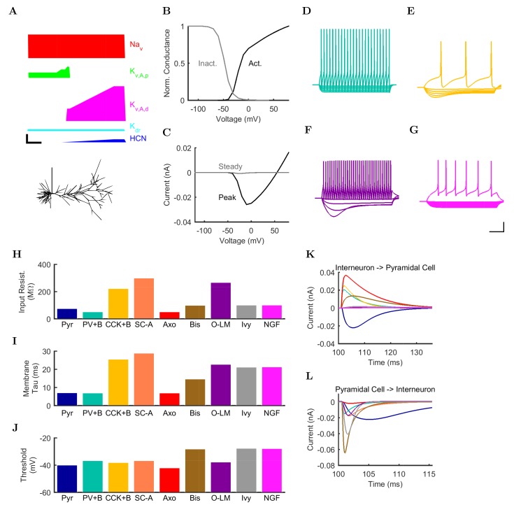
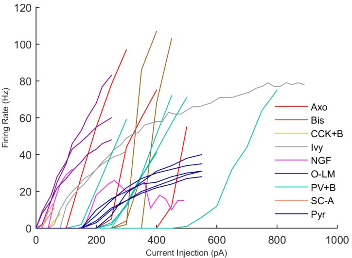
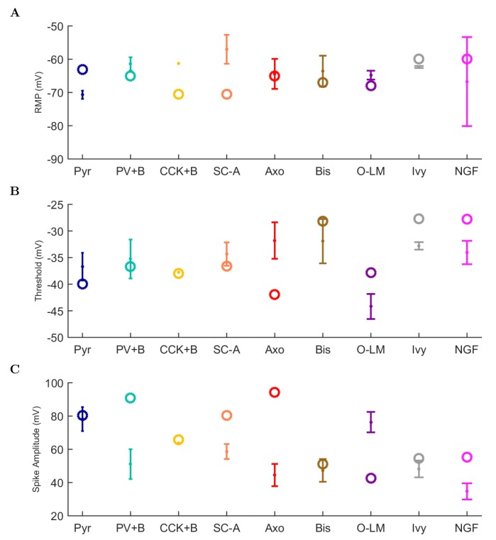
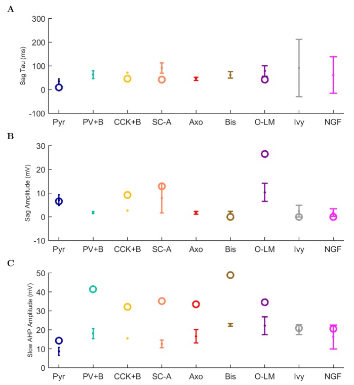
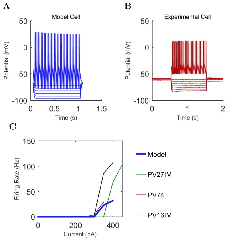
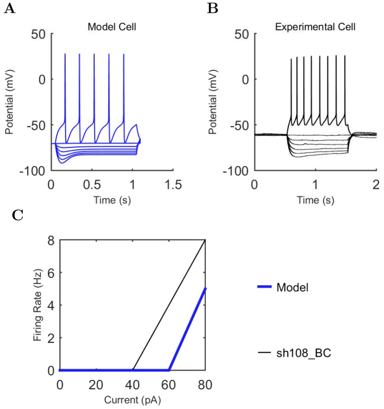
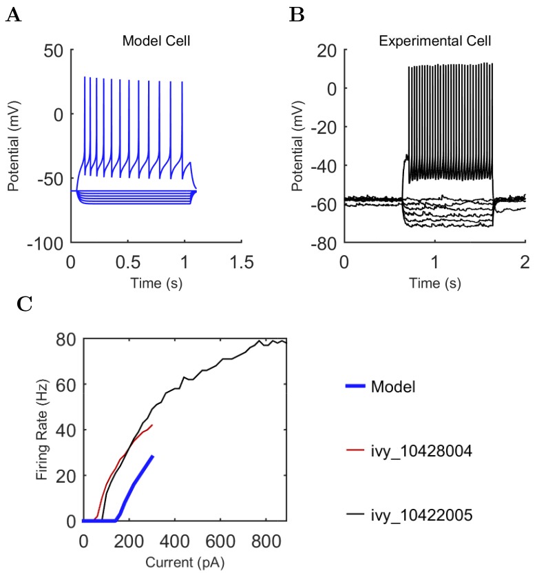
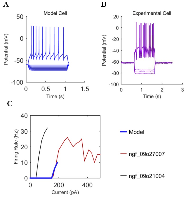
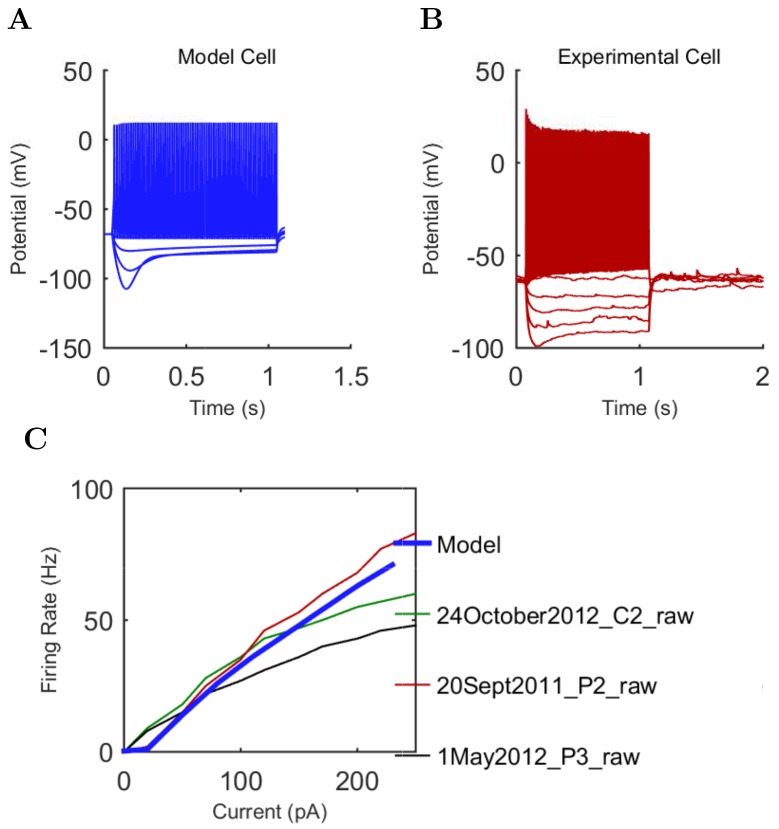
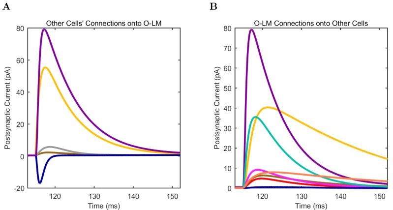
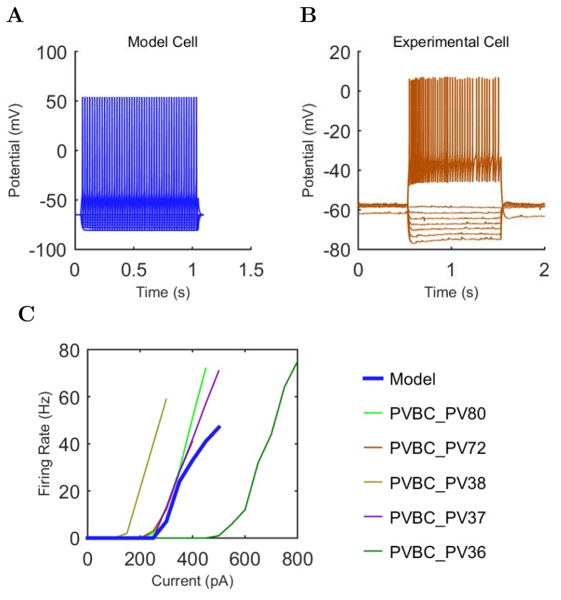
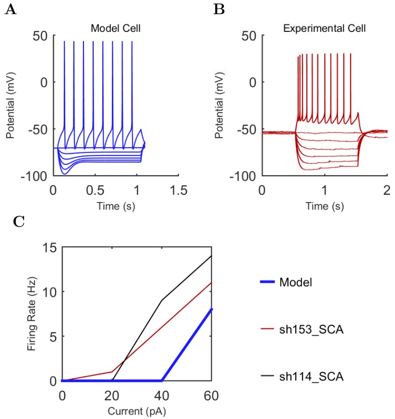
“The behavior of each cell type was characterized using a current injection sweep that matched experimental conditions reported in the literature”
§ Interneuronal mechanisms of hippocampal theta oscillations in a full-scale model of the rodent CA1 circuit > Materials and methods > Model development
plain- Asserted: passes — The authors put it forward as true.
- Checkable: passes — It can be checked against evidence.
- Load-bearing: fails — The paper’s conclusions may not depend on it.
- Based: passes — The paper gives a reason why it holds.
Probably not a substantial claim. The paper’s conclusions may not depend on it.
In the paper
“the in vivo theta rhythm has been reported to be either atropine resistant or atropine sensitive”
§ Interneuronal mechanisms of hippocampal theta oscillations in a full-scale model of the rodent CA1 circuit > Discussion > Rationale for bases of comparison between modeling results with experimental data
What the sources say
- Not checked yetcites Kramis et al., 1975 source
hedged- Asserted: passes — The authors put it forward as true.
- Checkable: passes — It can be checked against evidence.
- Load-bearing: passes — The paper’s conclusions depend on it.
- Based: passes — The paper gives a reason why it holds.
Probably not a substantial claim.
What the paper did — it cites no source for this, so there is none to check. The quote shows it is in the paper.
In the paper
“To ensure the model cells exhibited robust biophysical behavior in a wide range of network conditions, we implemented a standard, thorough characterization strategy for each cell type”
§ Interneuronal mechanisms of hippocampal theta oscillations in a full-scale model of the rodent CA1 circuit > Materials and methods > Model development
plaindirect- Asserted: passes — The authors put it forward as true.
- Checkable: passes — It can be checked against evidence.
- Load-bearing: fails — The paper’s conclusions may not depend on it.
- Based: passes — The paper gives a reason why it holds.
Probably not a substantial claim. The paper’s conclusions may not depend on it.
A conclusion the paper draws from its own results — it cites no other source for it, so there is none to check. The quote shows it is in the paper.
In the paper
“We developed a flexible and biologically relevant model that uses computational resources efficiently”
§ Interneuronal mechanisms of hippocampal theta oscillations in a full-scale model of the rodent CA1 circuit > Discussion > An accessible approach to modeling that balances detail, scale, flexibility and performance
plain- Asserted: passes — The authors put it forward as true.
- Checkable: passes — It can be checked against evidence.
- Load-bearing: passes — The paper’s conclusions depend on it.
- Based: passes — The paper gives a reason why it holds.
Probably not a substantial claim. It may state two separate claims as one.
What the paper did — it cites no source for this, so there is none to check. The quote shows it is in the paper.
In the paper
“The published experimental data were compared side-by-side with model cell simulation results”
§ Interneuronal mechanisms of hippocampal theta oscillations in a full-scale model of the rodent CA1 circuit > Materials and methods > Model development
plaincorrelational- Asserted: passes — The authors put it forward as true.
- Checkable: passes — It can be checked against evidence.
- Load-bearing: fails — The paper’s conclusions may not depend on it.
- Based: passes — The paper gives a reason why it holds.
Probably not a substantial claim. The paper’s conclusions may not depend on it.
What the paper did — it cites no source for this, so there is none to check. The quote shows it is in the paper.
In the paper
“We performed reference simulations and LFP analog calculations with the inner radius set to 200 μm and 500 μm and obtained results identical with those in Figures 3 and 4 (where an inner radius of 100 μm was used), except for negligible increases in the theta oscillation power found in the LFP analog spectrogram”
§ Interneuronal mechanisms of hippocampal theta oscillations in a full-scale model of the rodent CA1 circuit > Materials and methods > LFP analog
plain- Asserted: passes — The authors put it forward as true.
- Checkable: passes — It can be checked against evidence.
- Load-bearing: fails — The paper’s conclusions may not depend on it.
- Based: passes — The paper gives a reason why it holds.
Probably not a substantial claim. The paper’s conclusions may not depend on it.
What the paper did — it cites no source for this, so there is none to check. The quote shows it is in the paper.
In the paper
“the stimulation patterns used in the present study were not representative of the information content thought to be carried via inputs from those areas”
§ Interneuronal mechanisms of hippocampal theta oscillations in a full-scale model of the rodent CA1 circuit > Materials and methods > Stimulation
plain- Asserted: passes — The authors put it forward as true.
- Checkable: passes — It can be checked against evidence.
- Load-bearing: passes — The paper’s conclusions depend on it.
- Based: passes — The paper gives a reason why it holds.
Probably not a substantial claim.
The paper relies on this without support.
The CA1 area is one of the most extensively studied brain regions, with abundant anatomical and electrophysiological data about its organization.
“Because the CA1 area is one of the most extensively studied brain regions, there are abundant anatomical and electrophysiological data about its organization, making it a logical choice for the development of a full-scale model.”
The paper relies on this without support.
The model parameters that could not be constrained by experimental data do not critically affect the model's conclusions.
“In addition, the remaining parameters that could not be constrained by experimental data were documented, with the assumptions used to arrive at them explicitly listed in Table 2 of Bezaire and Soltesz (2013) and additional parameter calculations described in the Appendix of the present paper, section 'Inhibitory connectivity'.”
The paper relies on this without support.
The missing 30% of interneurons do not qualitatively alter the generation of theta oscillations in the model.
“The remaining 30% of the interneurons were not included in the model due to paucity of quantitative data (Bezaire and Soltesz, 2013).”
The paper relies on this without support.
The experimental phase preferences from anesthetized rats are comparable to the model's conditions.
“Firing probability by cell type as a function of theta phase for (A) model and (B) experimental cells under anesthesia (histograms adapted with permission from Figure 2, Figure 5B left, and Figure 6F respectively from Klausberger and Somogyi, 2008; Fuentealba et al., 2008; Fuentealba et al., 2010).”
The paper relies on this without support.
The phase preferences of interneurons in anesthetized animals are comparable to those in the model's conditions for the purpose of validating the model.
“because no data are available on the phase preferential firing of morphologically identified interneurons from the isolated CA1 preparation, comparison is made here with results from anesthetized animals, from which the most complete data sets are available”
The paper relies on this without support.
The parameter space explored for low-diversity configurations is sufficient to conclude that interneuronal diversity is necessary for spontaneous theta oscillations.
“While we could not rule out a hypothetical theta regime somewhere in the parameter space of such low-diversity configurations, any theta solution space would likely be smaller and more elusive than we were able to determine in the control configuration (Figure 6A).”
The paper relies on this without support.
The phase of LFP theta recorded in the stratum radiatum is approximately 180 degrees out of phase with the pyramidal cell layer theta used in this paper.
“note that Ferguson and colleagues used LFP theta recorded in the stratum radiatum as reference, which is approximately 180 degrees out of phase with the pyramidal cell layer theta used in this paper”
The paper relies on this without support.
Model neurons sometimes behave much differently than expected when subjected to current sweep protocols or synaptic inputs that are outside the range of the original protocols used to construct the model.
“Model neurons sometimes behave much differently than expected when subjected to current sweep protocols or synaptic inputs that are outside the range of the original protocols used to construct the model”
The authors state this as an assumption.
All available incoming inhibitory synapses onto interneurons in a layer have an equal chance of being innervated by the available inhibitory boutons targeting interneurons in that layer.
“All available incoming inhibitory synapses onto interneurons in a layer have an equal chance of being innervated by the available inhibitory boutons targeting interneurons in that layer”
The paper relies on this without support.
There is no reported evidence for major, systematic differences in key parameters such as the phase specific firing of rat and mouse interneurons in vivo.
“there is no reported evidence for major, systematic differences in key parameters such as the phase specific firing of rat and mouse interneurons in vivo”
Claims other papers make about this one
Each is checked against this paper’s own text: does it say what the citing paper says it does?
The cited source says what the claim attributes to it.
In the citing paper
“Fast-spiking (FS) CA1 interneurons (classically referred to as “theta cells”53) have been mechanistically linked to the emergence of the LFP theta rhythm and the entrainment of pyramidal neurons in the hippocampus42,54–56.”
From Place and behavioral modulation of hippocampal neurons during immobility (2026) · cites this paper as [54]
Citations
Cites
Memory and the hippocampus: A synthesis from findings with rats, monkeys, and humans.
Squire, L. R. (1992) · Psychological Review · doi:10.1037/0033-295x.99.2.195 · Cited by 5,376
The origin of extracellular fields and currents — EEG, ECoG, LFP and spikes
Buzsáki, G., Anastassiou, C. A., & Koch, C. (2012) · Nature Reviews Neuroscience · doi:10.1038/nrn3241 · Cited by 4,225
Theta oscillations in the hippocampus
Buzsáki, G. (2002) · Neuron · doi:10.1016/s0896-6273(02)00586-x · Cited by 3,332
Beta-band oscillations—Signalling the status quo?
Engel, A. K., & Fries, P. (2010) · Current Opinion in Neurobiology · doi:10.1016/j.conb.2010.02.015 · Cited by 2,953
Rhythms for cognition: communication through coherence
Fries, P. (2015) · Neuron · doi:10.1016/j.neuron.2015.09.034 · Cited by 2,725
Neuronal Diversity and Temporal Dynamics: The Unity of Hippocampal Circuit Operations
Klausberger, T., & Somogyi, P. (2008) · Science · doi:10.1126/science.1149381 · Cited by 2,050
Place Cells, Grid Cells, and the Brain's Spatial Representation System
Moser, E. I., Kropff, E., & Moser, M.-B. (2008) · Annual Review of Neuroscience · doi:10.1146/annurev.neuro.31.061307.090723 · Cited by 1,934
Memory, navigation and theta rhythm in the hippocampal-entorhinal system
Buzsáki, G., & Moser, E. I. (2013) · Nature Neuroscience · doi:10.1038/nn.3304 · Cited by 1,847
Lisman, J. E., & Jensen, O. (2013) · Neuron · doi:10.1016/j.neuron.2013.03.007 · Cited by 1,609
Reconstruction and Simulation of Neocortical Microcircuitry
Markram, H., Muller, E., Ramaswamy, S., Reimann, M. W., Abdellah, M., Sanchez, C. A., Ailamaki, A., Alonso-Nanclares, L., Antille, N., Arsever, S., et al. (2015) · Cell · doi:10.1016/j.cell.2015.09.029 · Cited by 1,557
Cited by
Sorted by citations
Illuminating dendritic function with computational models
Poirazi, P., & Papoutsi, A. (2020) · Nature reviews. Neuroscience · doi:10.1038/s41583-020-0301-7 · Cited by 313
Inhibitory Interneurons Regulate Temporal Precision and Correlations in Cortical Circuits
Cardin, J. A. (2018) · Trends in Neurosciences · doi:10.1016/j.tins.2018.07.015 · Cited by 254
Turi, G. F., Li, W.-K., Chavlis, S., Pandi, I., O’Hare, J., Priestley, J. B., Grosmark, A. D., Liao, Z., Ladow, M., Zhang, J. F., et al. (2019) · Neuron · doi:10.1016/j.neuron.2019.01.009 · Cited by 218
Breakdown of spatial coding and interneuron synchronization in epileptic mice
Shuman, T., Aharoni, D. B., Cai, D. J., Lee, C. R., Chavlis, S., Page-Harley, L., Vetere, L. M., Feng, Y., Yang, C. Y., Mollinedo-Gajate, I., et al. (2020) · Nature Neuroscience · doi:10.1038/s41593-019-0559-0 · Cited by 198
The Neurodata Without Borders ecosystem for neurophysiological data science
Rübel, O., Tritt, A., Ly, R., Dichter, B., Ghosh, S., Niu, L., Baker, P. M., Soltész, I., Ng, L., Svoboda, K., et al. (2022) · eLife · doi:10.7554/elife.78362 · Cited by 201
NetPyNE, a tool for data-driven multiscale modeling of brain circuits
Dura-Bernal, S., Suter, B. A., Gleeson, P., Cantarelli, M., Quintana, A., Rodriguez, F., Kedziora, D. J., Chadderdon, G. L., Kerr, C. C., Neymotin, S. A., et al. (2019) · eLife · doi:10.7554/elife.44494 · Cited by 169
The role of inhibitory circuits in hippocampal memory processing
Topolnik, L., & Tamboli, S. (2022) · Nature reviews. Neuroscience · doi:10.1038/s41583-022-00599-0 · Cited by 165
Schulz, J. M., Knoflach, F., Hernandez, M., & Bischofberger, J. (2018) · Nature Communications · doi:10.1038/s41467-018-06004-8 · Cited by 128
Visualization of currents in neural models with similar behavior and different conductance densities
Alonso, L. M., & Marder, E. (2019) · eLife · doi:10.7554/elife.42722 · Cited by 119
Challenging the point neuron dogma: FS basket cells as 2-stage nonlinear integrators
Tzilivaki, A., Kastellakis, G., & Poirazi, P. (2019) · Nature Communications · doi:10.1038/s41467-019-11537-7 · Cited by 115
Gleeson, P., Cantarelli, M., Marin, B., Quintana, A., Earnshaw, M., Sadeh, S., Piasini, E., Birgiolas, J., Cannon, R. C., Cayco-Gajic, N. A., et al. (2019) · Neuron · doi:10.1016/j.neuron.2019.05.019 · Cited by 87
Navas-Olivé, A., Valero, M., Jurado-Parras, T., de Salas-Quiroga, A., Averkin, R. G., Gambino, G., Cid, E., & de la Prida, L. M. (2020) · Nature Communications · doi:10.1038/s41467-020-15840-6 · Cited by 80
Brain Modeling ToolKit: An open source software suite for multiscale modeling of brain circuits
Dai, K., Gratiy, S. L., Billeh, Y. N., Xu, R., Cai, B., Cain, N., Rimehaug, A. E., Stasik, A. J., Einevoll, G. T., Mihalaş, Ş., et al. (2020) · PLoS Computational Biology · doi:10.1371/journal.pcbi.1008386 · Cited by 72
Degeneracy in epilepsy: multiple routes to hyperexcitable brain circuits and their repair
Stöber, T. M., Batulin, D., Triesch, J., Narayanan, R., & Jedlička, P. (2023) · Communications Biology · doi:10.1038/s42003-023-04823-0 · Cited by 65
Nicola, W., & Clopath, C. (2019) · Nature Neuroscience · doi:10.1038/s41593-019-0415-2 · Cited by 61
Chittajallu, R., Wester, J. C., Craig, M. T., Barksdale, E., Yuan, X. Q., Akgül, G., Fang, C., Collins, D., Hunt, S., Pelkey, K. A., et al. (2017) · Nature Communications · doi:10.1038/s41467-017-00218-y · Cited by 58
Data‐driven integration of hippocampal CA1 synaptic physiology in silico
Ecker, A., Romani, A., Sáray, S., Káli, S., Migliore, M., Falck, J. E., Lange, S., Mercer, A., Thomson, A. M., Muller, E. B., et al. (2020) · Hippocampus · doi:10.1002/hipo.23220 · Cited by 55
Resolving the Micro-Macro Disconnect to Address Core Features of Seizure Networks
Farrell, J. S., Nguyen, Q.-A., & Soltész, I. (2019) · Neuron · doi:10.1016/j.neuron.2019.01.043 · Cited by 56
BioNet: A Python interface to NEURON for modeling large-scale networks
Gratiy, S. L., Billeh, Y. N., Dai, K., Mitelut, C., Feng, D. H., Gouwens, N. W., Cain, N., Koch, C., Anastassiou, C. A., & Arkhipov, A. S. (2018) · PLoS ONE · doi:10.1371/journal.pone.0201630 · Cited by 53
Solving brain circuit function and dysfunction with computational modeling and optogenetic fMRI
Lee, J. H., Liu, Q., & Dadgar‐Kiani, E. (2022) · Science · doi:10.1126/science.abq3868 · Cited by 59
Quantitative firing pattern phenotyping of hippocampal neuron types
Komendantov, A. O., Venkadesh, S., Rees, C. L., Wheeler, D. W., Hamilton, D. J., & Ascoli, G. A. (2019) · Scientific Reports · doi:10.1038/s41598-019-52611-w · Cited by 52
Liu, Z., Han, F., & Wang, Q. (2022) · Nonlinear Dynamics · doi:10.1007/s11071-022-07298-6 · Cited by 52
Inhibition shapes the organization of hippocampal representations
McKenzie, S. (2017) · Hippocampus · doi:10.1002/hipo.22803 · Cited by 46
Bilash, O. M., Chavlis, S., Johnson, C. D., Poirazi, P., & Basu, J. (2023) · Cell Reports · doi:10.1016/j.celrep.2022.111962 · Cited by 52
Mehak, S. F., Shivakumar, A. B., Kumari, S., Muralidharan, B., & Gangadharan, G. (2022) · Neuroscience & Biobehavioral Reviews · doi:10.1016/j.neubiorev.2022.104628 · Cited by 45
Active Dendrites and Local Field Potentials: Biophysical Mechanisms and Computational Explorations
Sinha, M., & Narayanan, R. (2021) · Neuroscience · doi:10.1016/j.neuroscience.2021.08.035 · Cited by 44
Feng, F., Headley, D. B., Amir, A., Kanta, V., Chen, Z., Paré, D., & Nair, S. S. (2019) · eNeuro · doi:10.1523/eneuro.0388-18.2018 · Cited by 45
Attili, S. M., Silva, M. F. M., Nguyen, T.-V., & Ascoli, G. A. (2019) · Brain Structure and Function · doi:10.1007/s00429-019-01940-7 · Cited by 35
Parallel odor processing by mitral and middle tufted cells in the olfactory bulb
Cavarretta, F., Burton, S. D., Igarashi, K. M., Shepherd, G. M., Hines, M. L., & Migliore, M. (2018) · Scientific Reports · doi:10.1038/s41598-018-25740-x · Cited by 33
Novel long-range inhibitory nNOS-expressing hippocampal cells
Wick, Z. C., Tetzlaff, M. R., & Krook-Magnuson, E. I. (2019) · eLife · doi:10.7554/elife.46816 · Cited by 37
Inhibitory conductance controls place field dynamics in the hippocampus
Valero, M., Navas-Olivé, A., de la Prida, L. M., & Buzsáki, G. (2022) · Cell Reports · doi:10.1016/j.celrep.2022.111232 · Cited by 39
Romani, A., Antonietti, A., Bella, D., Budd, J., Giacalone, E., Kurban, K., Sáray, S., Abdellah, M., Arnaudon, A., Boci, E., et al. (2024) · PLOS Biology · doi:10.1371/journal.pbio.3002861 · Cited by 39
Venkadesh, S., Komendantov, A. O., Wheeler, D. W., Hamilton, D. J., & Ascoli, G. A. (2019) · PLoS Computational Biology · doi:10.1371/journal.pcbi.1007462 · Cited by 32
Kang, Y., Clement, E. M., Park, I., Greenfield, L. J., Smith, B. N., & Lee, S.-H. (2021) · Experimental Neurology · doi:10.1016/j.expneurol.2021.113724 · Cited by 31
Full-scale scaffold model of the human hippocampus CA1 area
Gandolfi, D., Mapelli, J., Solinas, S. M. G., Triebkorn, P., D'Angelo, E. U., Jirsa, V., & Migliore, M. (2023) · Nature Computational Science · doi:10.1038/s43588-023-00417-2 · Cited by 31
Hernández‐Frausto, M., Bilash, O. M., Masurkar, A. V., & Basu, J. (2023) · Frontiers in Neural Circuits · doi:10.3389/fncir.2023.1223891 · Cited by 35
Durá-Bernal, S., Griffith, E. Y., Barczak, A., O’Connell, M. N., McGinnis, T., Moreira, J. V. S., Schroeder, C. E., Lytton, W. W., Lakatos, P., & Neymotin, S. A. (2023) · Cell Reports · doi:10.1016/j.celrep.2023.113378 · Cited by 36
Chatzikalymniou, A. P., & Skinner, F. K. (2018) · eNeuro · doi:10.1523/eneuro.0146-18.2018 · Cited by 32
Integrative Models of Brain Structure and Dynamics: Concepts, Challenges, and Methods
Venkadesh, S., & Horn, J. D. V. (2021) · Frontiers in Neuroscience · doi:10.3389/fnins.2021.752332 · Cited by 25
Single Bursts of Individual Granule Cells Functionally Rearrange Feedforward Inhibition
Neubrandt, M., Oláh, V. J., Brunner, J., Marosi, E. L., Soltész, I., & Szabadics, J. (2018) · Journal of Neuroscience · doi:10.1523/jneurosci.1595-17.2018 · Cited by 28
Sáray, S., Rössert, C., Appukuttan, S., Migliore, R., Vitale, P., Lupaşcu, C. A., Bologna, L. L., Geit, W. A. H. V., Romani, A., Davison, A. P., et al. (2021) · PLoS Computational Biology · doi:10.1371/journal.pcbi.1008114 · Cited by 27
Ferguson, K., Chatzikalymniou, A. P., & Skinner, F. K. (2017) · eNeuro · doi:10.1523/eneuro.0131-17.2017 · Cited by 27
Wal, M. T., & Tiesinga, P. H. E. (2021) · Biological Cybernetics · doi:10.1007/s00422-021-00894-6 · Cited by 27
From mechanisms to functions: The role of theta and gamma coherence in the intrahippocampal circuits
Mysin, I. E., & Shubina, L. (2022) · Hippocampus · doi:10.1002/hipo.23410 · Cited by 31
Theta-gamma phase amplitude coupling in a hippocampal CA1 microcircuit
Ponzi, A. P. D., Durá-Bernal, S., & Migliore, M. (2023) · PLoS Computational Biology · doi:10.1371/journal.pcbi.1010942 · Cited by 23
A comprehensive knowledge base of synaptic electrophysiology in the rodent hippocampal formation
Moradi, K., & Ascoli, G. A. (2019) · Hippocampus · doi:10.1002/hipo.23148 · Cited by 22
Mysin, I. E., Kitchigina, V. F., & Kazanovich, Y. B. (2019) · Neural Networks · doi:10.1016/j.neunet.2019.04.004 · Cited by 23
Kopsick, J. D., Tecuatl, C., Moradi, K., Attili, S. M., Kashyap, H. J., Xing, J., Chen, K., Krichmar, J. L., & Ascoli, G. A. (2022) · Cognitive Computation · doi:10.1007/s12559-021-09954-2 · Cited by 22
Offline memory replay in recurrent neuronal networks emerges from constraints on online dynamics
Milstein, A. D., Tran, S., Ng, G. Y., & Soltész, I. (2022) · The Journal of Physiology · doi:10.1113/jp283216 · Cited by 24
On the structural connectivity of large-scale models of brain networks at cellular level
Giacopelli, G., Tegolo, D., Spera, E., & Migliore, M. (2021) · Scientific Reports · doi:10.1038/s41598-021-83759-z · Cited by 26
Large-scale biophysically detailed model of somatosensory thalamocortical circuits in NetPyNE
Borges, F. S., Moreira, J. V. S., Takarabe, L. M., Lytton, W. W., & Durá-Bernal, S. (2022) · Frontiers in Neuroinformatics · doi:10.3389/fninf.2022.884245 · Cited by 23
Integrating multimodal data to understand cortical circuit architecture and function
Arkhipov, A. S., da Costa, N. M., de Vries, S. E. J., Bakken, T. E., Bennett, C., Bernard, A., Berg, J., Buice, M. A., Collman, F., Daigle, T. L., et al. (2025) · Nature Neuroscience · doi:10.1038/s41593-025-01904-7 · Cited by 27
Attili, S. M., Moradi, K., Wheeler, D. W., & Ascoli, G. A. (2022) · European Journal of Neuroscience · doi:10.1111/ejn.15639 · Cited by 26
Data-driven multiscale computational models of cortical and subcortical regions
Ramaswamy, S. (2024) · Current Opinion in Neurobiology · doi:10.1016/j.conb.2024.102842 · Cited by 22
Multi-scale spiking network model of human cerebral cortex
Pronold, J., van Meegen, A., Shimoura, R. O., Vollenbröker, H., Senden, M., Hilgetag, C. C., Bakker, R., & van Albada, S. J. (2024) · Cerebral Cortex · doi:10.1093/cercor/bhae409 · Cited by 26
Estimation of neural network model parameters from local field potentials (LFPs)
Skaar, J.-E. W., Stasik, A., Hagen, E., Ness, T. V., & Einevoll, G. T. (2020) · PLoS Computational Biology · doi:10.1371/journal.pcbi.1007725 · Cited by 20
NeuroML-DB: Sharing and characterizing data-driven neuroscience models described in NeuroML
Birgiolas, J., Haynes, V., Gleeson, P., Gerkin, R. C., Dietrich, S. W., & Crook, S. M. (2023) · PLoS Computational Biology · doi:10.1371/journal.pcbi.1010941 · Cited by 23
Quantitative simulation of extracellular single unit recording from the surface of cortex
Hill, M., Rios, E., Sudhakar, S., Roossien, D. H., Caldwell, C. M., Cai, D., Ahmed, O. J., Lempka, S. F., & Chestek, C. A. (2018) · Journal of Neural Engineering · doi:10.1088/1741-2552/aacdb8 · Cited by 19
Learning, Fast and Slow: Single- and Many-Shot Learning in the Hippocampus
Liao, Z., & Losonczy, A. (2024) · Annual Review of Neuroscience · doi:10.1146/annurev-neuro-102423-100258 · Cited by 26
Reconstruction of the Hippocampus
Romani, A., Schürmann, F., Markram, H., & Migliore, M. (2022) · Advances in experimental medicine and biology · doi:10.1007/978-3-030-89439-9_11 · Cited by 18
Cell Type-specific Intrinsic Perithreshold Oscillations in Hippocampal GABAergic Interneurons
Kang, Y., Lewis, H. E. S., Young, M. W., Govindaiah, G., Greenfield, L. J., García‐Rill, E., & Lee, S.-H. (2018) · Neuroscience · doi:10.1016/j.neuroscience.2018.02.014 · Cited by 16
Ultrafast simulation of large-scale neocortical microcircuitry with biophysically realistic neurons
Oláh, V. J., Pedersen, N. P., & Rowan, M. J. (2022) · eLife · doi:10.7554/elife.79535 · Cited by 15
Zhou, H., Zhu, J., Jia, J., Xiang, W., Peng, H., Zhang, Y., Liu, B., Mu, Y., & Lu, Y. (2022) · Neurobiology of Stress · doi:10.1016/j.ynstr.2022.100492 · Cited by 19
Noguchi, A., Yamashiro, K., Matsumoto, N., & Ikegaya, Y. (2023) · Communications Biology · doi:10.1038/s42003-023-04719-z · Cited by 17
Network instability dynamics drive a transient bursting period in the developing hippocampus in vivo
Graf, J., Rahmati, V., Majoros, M., Witte, O. W., Geis, C., Kiebel, S. J., Holthoff, K., & Kirmse, K. (2022) · eLife · doi:10.7554/elife.82756 · Cited by 15
Schumm, S. N., Gabrieli, D. J., & Meaney, D. F. (2022) · Hippocampus · doi:10.1002/hipo.23402 · Cited by 15
Durá-Bernal, S., Griffith, E. Y., Barczak, A., O’Connell, M. N., McGinnis, T., Schroeder, C. E., Lytton, W. W., Lakatos, P., & Neymotin, S. A. (2022) · bioRxiv (Cold Spring Harbor Laboratory) · doi:10.1101/2022.02.03.479036 · Cited by 16
Linaro, D., Levy, M. J., & Hunt, D. L. (2022) · PLoS Computational Biology · doi:10.1371/journal.pcbi.1010071 · Cited by 22
Functional specification of CCK+ interneurons by alternative isoforms of Kv4.3 auxiliary subunits
Oláh, V. J., Lukacsovich, D., Winterer, J., Arszovszki, A., Lőrincz, A., Nusser, Z., Földy, C., & Szabadics, J. (2020) · eLife · doi:10.7554/elife.58515 · Cited by 14
Tsolias, A., & Medalla, M. (2022) · Frontiers in Neural Circuits · doi:10.3389/fncir.2021.795325 · Cited by 13
The potential role of the cholecystokinin system in declarative memory
Lau, S. H., Young, C. H., Zheng, Y., & Chen, X. (2022) · Neurochemistry International · doi:10.1016/j.neuint.2022.105440 · Cited by 16
Adaikkan, C., Joseph, J., Foustoukos, G., Wang, J., Polygalov, D., Boehringer, R., Middleton, S. J., Huang, A. J. Y., Tsai, L., & McHugh, T. J. (2024) · Nature Communications · doi:10.1038/s41467-024-46478-3 · Cited by 16
Inhibitory plasticity supports replay generalization in the hippocampus
Liao, Z., Terada, S., Raikov, I., Hadjiabadi, D. H., Szoboszlay, M., Soltész, I., & Losonczy, A. (2024) · Nature Neuroscience · doi:10.1038/s41593-024-01745-w · Cited by 14
Self-citationDo Process-1 simulations generate the epistemic feelings that drive Process-2 decision making?
Fields, C., & Glazebrook, J. F. (2020) · Cognitive Processing · doi:10.1007/s10339-020-00981-9 · Cited by 14
Braun, W., & Memmesheimer, R.-M. (2022) · PLoS Computational Biology · doi:10.1371/journal.pcbi.1009891 · Cited by 14
Chatzikalymniou, A. P., Gumus, M., Lunyov, A. R., Rich, S., Lefebvre, J., & Skinner, F. K. (2021) · Hippocampus · doi:10.1002/hipo.23364 · Cited by 13
Wheeler, D. W., Kopsick, J. D., Sutton, N. M., Tecuatl, C., Komendantov, A. O., Nadella, K., & Ascoli, G. A. (2023) · eLife · doi:10.7554/elife.90597 · Cited by 14
Földi, T., Lörincz, M. L., & Berényi, A. (2021) · Frontiers in Neural Circuits · doi:10.3389/fncir.2021.784085 · Cited by 14
Gandolfi, D., Mapelli, J., Solinas, S. M. G., Schepper, R. D., Geminiani, A., Casellato, C., D'Angelo, E. U., & Migliore, M. (2022) · Scientific Reports · doi:10.1038/s41598-022-18024-y · Cited by 13
Multinode implementation of an extended Hodgkin–Huxley simulator
Chatzikonstantis, G., Sidiropoulos, H., Strydis, C., Negrello, M., Smaragdos, G., Zeeuw, C. I. D., & Soudris, D. (2018) · Neurocomputing · doi:10.1016/j.neucom.2018.10.062 · Cited by 15
Sendi, M. S. E., Inman, C. S., Bijanki, K. R., Blanpain, L. T., Park, J. K., Hamann, S. B., Gross, R. E., Willie, J. T., & Mahmoudi, B. (2021) · Brain stimulation · doi:10.1016/j.brs.2021.09.009 · Cited by 13
Theta-phase locking of single neurons during human spatial memory
Guth, T. A., Brandt, A., Reinacher, P. C., Schulze‐Bonhage, A., Jacobs, J., & Kunz, L. (2025) · Nature Communications · doi:10.1038/s41467-025-62553-9 · Cited by 15
Computational models of memory consolidation and long-term synaptic plasticity during sleep
Rennó‐Costa, C., da Silva, A. C. C., Blanco, W., & Ribeiro, S. T. G. (2018) · Neurobiology of Learning and Memory · doi:10.1016/j.nlm.2018.10.003 · Cited by 12
Sutton, N. M., & Ascoli, G. A. (2021) · Cognitive Systems Research · doi:10.1016/j.cogsys.2021.07.008 · Cited by 12
Medalla, M., Chang, W., Ibañez, S., Guillamón-Vivancos, T., Nittmann, M., Kapitonava, A., Busch, S. E., Moore, T. L., Rosene, D. L., & Luebke, J. I. (2021) · Cerebral Cortex · doi:10.1093/cercor/bhab347 · Cited by 13
Vardalakis, N., Aussel, A., Rougier, N. P., & Wagner, F. B. (2023) · eLife · doi:10.7554/elife.87356 · Cited by 13
Sutton, N. M., Gutiérrez-Guzmán, B. E., Dannenberg, H., & Ascoli, G. A. (2024) · International Journal of Molecular Sciences · doi:10.3390/ijms25116059 · Cited by 14
Wei, X., Campagna, J. J., Jagodzinska, B. M., Wi, D., Cohn, W., Lee, J. T., Zhu, C., Huang, C., Molnár, L., Houser, C. R., et al. (2024) · Proceedings of the National Academy of Sciences · doi:10.1073/pnas.2400420121 · Cited by 15
Osanai, H., Nair, I. R., & 北村, 貴. (2023) · Journal of Neurochemistry · doi:10.1111/jnc.15850 · Cited by 16
Hasselmo, M. E., Alexander, A. S., Hoyland, A., Robinson, J. C., Bezaire, M. J., Chapman, G. W., Saudargienė, A., Carstensen, L. C., & Dannenberg, H. (2020) · Neuroscience · doi:10.1016/j.neuroscience.2020.03.048 · Cited by 11
Self-citationHypothalamic regulation of hippocampal CA1 interneurons by the supramammillary nucleus
Jiang, Y., Lee, D. K., Guo, W., Li, M., & Sun, Q. (2024) · Cell Reports · doi:10.1016/j.celrep.2024.114898 · Cited by 10
Dainauskas, J. J., Marie, H., Migliore, M., & Saudargienė, A. (2023) · Frontiers in Synaptic Neuroscience · doi:10.3389/fnsyn.2023.1113957 · Cited by 10
The critical role of persistent sodium current in hippocampal gamma oscillations
Kang, Y., Clement, E. M., Sumsky, S. L., Xiang, Y., Park, I., Santaniello, S., Greenfield, L. J., García‐Rill, E., Smith, B. N., & Lee, S.-H. (2019) · Neuropharmacology · doi:10.1016/j.neuropharm.2019.107787 · Cited by 11
Ozsvár, A., Komlósi, G., Oláh, G., Baka, J., Molnár, G., & Tamás, G. (2021) · eLife · doi:10.7554/elife.65634 · Cited by 8
Guet-McCreight, A., & Skinner, F. K. (2019) · PLoS ONE · doi:10.1371/journal.pone.0209429 · Cited by 11
Regulation of gamma‐frequency oscillation by feedforward inhibition: A computational modeling study
Rennó‐Costa, C., Teixeira, D. G., & Soltész, I. (2019) · Hippocampus · doi:10.1002/hipo.23093 · Cited by 9
The SONATA Data Format for Efficient Description of Large-Scale Network ModelsPreprint
Dai, K., Hernando, J., Billeh, Y. N., Gratiy, S. L., Planas, J., Davison, A. P., Durá-Bernal, S., Gleeson, P., Devresse, A., Dichter, B., et al. (2019) · bioRxiv (Cold Spring Harbor Laboratory) · doi:10.1101/625491 · Cited by 10
Spiral wave dynamics in a neuronal network model
Souza, D. L. M., Borges, F. S., Gabrick, E. C., Bentivoglio, L. E., Protachevicz, P. R., dos Santos, V., Viana, R. L., Caldas, I. L., Iarosz, K. C., Batista, A. M., et al. (2024) · Journal of Physics Complexity · doi:10.1088/2632-072x/ad42f6 · Cited by 9
Hippocampal interneuronal dysfunction and hyperexcitability in a porcine model of concussion
Ulyanova, A. V., Adam, C. D., Cottone, C., Maheshwari, N., Grovola, M. R., Fruchet, O., Alamar, J., Koch, P. F., Johnson, V. E., Cullen, D. K., et al. (2023) · Communications Biology · doi:10.1038/s42003-023-05491-w · Cited by 12
Memory Prosthesis: Is It Time for a Deep Neuromimetic Computing Approach?
Cutsuridis, V. (2019) · Frontiers in Neuroscience · doi:10.3389/fnins.2019.00667 · Cited by 10
Metadata
- Authors
- Bezaire, M. J., Raikov, I., Burk, K., Vyas, D., & Soltesz, I.
- Affiliations
- University of California, Irvine (US)
- Department of Neurosurgery, Stanford University, Stanford, United States
- Venue
- eLife
- Publisher
- eLife Sciences Publications, Ltd
- Published
- 2016-12-23
- Volume
- 5
- ISSN
- 2050-084X (ISSN-L)
- PMC
- PMC5313080
- OpenAlex
- W2561068888
- Semantic Scholar
- bf83b20cd9cedc55b96997bba3dd31b6cb9f1231
- Cited by
- 198
- References
- 160
- Citations by year
- 2026: 8 · 2025: 16 · 2024: 27 · 2023: 26 · 2022: 32 · 2021: 25 · 2020: 15 · 2019: 28 · 2018: 15 · 2017: 5 · 2016: 1
- FWCI
- 10.39
- Type
- journal article
- Language
- en
- Open access
- gold
- doi.org
- Licence
- Locations
- eLife (publishedVersion, cc-by)
- bioRxiv (Cold Spring Harbor Laboratory) (acceptedVersion, cc-by)
- Europe PMC (PubMed Central) (publishedVersion, cc-by)
- PubMed Central (publishedVersion, cc-by)
- PubMed (publishedVersion)
- DOAJ (DOAJ: Directory of Open Access Journals) (submittedVersion, cc-by-sa)
- Funders
- National Institutes of Health (F32NS090753, NS35915, NS090583)
- National Science Foundation (DGE-0808392, XSEDE Allocations - TG-IBN140007, XSEDE Allocations - TG-IBN130022, XSEDE Allocations - TG-IBN100011, IOS-1310378)
- Topics
- Life Sciences › Neuroscience › Cognitive Neuroscience › Neural dynamics and brain function
- Life Sciences › Neuroscience › Cognitive Neuroscience › Memory and Neural Mechanisms
- Life Sciences › Neuroscience › Cellular and Molecular Neuroscience › Neuroscience and Neuropharmacology Research
- Keywords
- hippocampal theta rhythm, interneurons, parvalbumin interneurons, neurogliaform cells, gamma oscillations, phase locking, computational neuroscience, spontaneous oscillations
- MeSH terms
- Animals, Interneurons, Neuroglia, Theta Rhythm, Neural Networks, Computer, Mice, Rats, CA1 Region, Hippocampal, Spatio-Temporal Analysis
About these checks
Registry, retraction, Cites and statistics results are computed, not judged, with one exception: a printed reference that no index lists is read once by a model before it counts as a citation error. Claims are extracted by a model and kept only when their quote appears verbatim in the text; each cited source is then checked, with a model’s help, for whether it says what the claim relies on. Those verdicts can be wrong — read the claim’s quote and the cited source before relying on one.
A language model drew the claims from the paper on 2026-10-09, under version 3 of the claim definition (model deepseek-v4.1-flash, prompt extract-v3).
A second model labelled each claim on 2026-10-09 (model jev-1.13-20260917, definition revision gold-guideline-v0.2).
Statistics and arithmetic are recomputed, not judged.
Confidence bands are shown only for fields calibrated on our annotated test set. None is calibrated yet, so no band is shown.
What counts as a claim ›How we measure confidence ›How we check this ›
Are you an author, or do you see a problem with this page? Request a review
