

The DOI matches its Crossref record; 62 of the 62 references it cites were found in a registry or an index; 24 of the 53 sources its claims cite were checked for support.
Citizen science charts two major “stomatotypes” in the oral microbiome of adolescents and reveals links with habits and drinking water composition
Open accessAbstract
BACKGROUND: The oral cavity comprises a rich and diverse microbiome, which plays important roles in health and disease. Previous studies have mostly focused on adult populations or in very young children, whereas the adolescent oral microbiome remains poorly studied. Here, we used a citizen science approach and 16S profiling to assess the oral microbiome of 1500 adolescents around Spain and its relationships with lifestyle, diet, hygiene, and socioeconomic and environmental parameters. RESULTS: Our results provide a detailed snapshot of the adolescent oral microbiome and how it varies with lifestyle and other factors. In addition to hygiene and dietary habits, we found that the composition of tap water was related to important changes in the abundance of several bacterial genera. This points to an important role of drinking water in shaping the oral microbiota, which has been so far poorly explored. Overall, the microbiome samples of our study can be clustered into two broad compositional patterns (stomatotypes), driven mostly by Neisseria and Prevotella, respectively. These patterns show striking similarities with those found in unrelated populations. CONCLUSIONS: We hypothesize that these stomatotypes represent two possible global optimal equilibria in the oral microbiome that reflect underlying constraints of the human oral niche. As such, they should be found across a variety of geographical regions, lifestyles, and ages.
Overview
AI snapshot
Written from the paper’s full text.
TL;DR
A citizen-science 16S survey of 1,319 Spanish adolescents found that oral microbiomes cluster into two broad “stomatotypes” driven mainly by Neisseria and Prevotella, with parallels to unrelated adult populations. Tap water chemistry was the investigated factor most strongly associated with changes in several oral genera, while hygiene, diet, and lifestyle showed more limited links.
Key findings
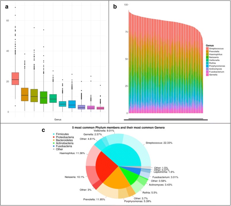
- From 1,555 collected samples, 1,319 passed quality filters; 332 genera-level OTUs were identified, with 32 genera present in ≥75% of individuals. The top ten genera made up 84.64% of sequences and appeared in 99.6% of samples; Streptococcus was most abundant in 68% of samples (mean 22.3%), followed by Prevotella (11.9%), Haemophilus (11.4%), Neisseria (10.1%), and Veillonella (9%).
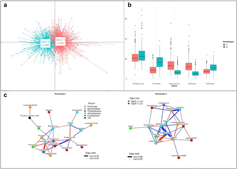
- Samples clustered into two stomatotypes: stomatotype 1 driven by Neisseria and stomatotype 2 driven by Prevotella, with higher Haemophilus in stomatotype 1 and higher Veillonella and Streptococcus in stomatotype 2. The authors note similarities to two “coinhabiting groups” in a Japanese adult study and propose naming them Neisseria-Haemophilus and Prevotella-Veillonella stomatotypes.
- Tap water composition was linked to oral microbiome variation: among 17 water parameters, Porphyromonas was positively associated with fluoride and sulfate, while Veillonella, Ralstonia, Rhizobium, Rhodococcus, and Pseudomonas negatively correlated with hardness, alkalinity, conductivity, sulfate, magnesium, sodium, calcium, chloride, and dry matter after boiling.
- Hygiene and habits had measurable but narrower associations: brushing frequency negatively correlated with Gemella, Streptobacillus, Granulicatella, and Porphyromonas; braces correlated positively with many genera; alcohol consumption among 314 students was associated with higher Mycoplasma, Filifactor, Treponema, and Desulfobulbus, while 108 students who smoked showed no significant microbiome differences.
Methods
- Citizen-science sampling of adolescents ages 13–15 and their teachers in 40 Spanish schools during Spring 2015, using oral rinse samples, a 54-question questionnaire, and saliva pH measured with test strips.
- DNA was extracted and the V3–V4 regions of 16S rRNA were sequenced on Illumina MiSeq; reads were processed with Mothur v1.34.4, SILVA v119 alignment, and genus-level OTU grouping.
- Microbiome composition was analyzed in R with Phyloseq; stomatotypes were defined by PAM clustering across five beta-diversity measures, with JSD used for main analyses, and associations tested using Pearson correlations, Kruskal-Wallis, ANOVA/TukeyHSD, chi-squared tests, and Bonferroni correction.
Limitations
- The paper states that citizen science limits comprehensive clinical evaluation by experts, that saliva pH strips lack pH-meter precision, and that low-abundance genera may reflect sporadic environmental colonization rather than stable oral residents.
- The paper notes that adolescents may have recently adopted some habits, so effects of smoking or diet may not yet be apparent, and that stomatotypes represent trends along a continuous gradient rather than discrete, well-separated entities.
- The text makes evident that time since last tooth brushing was not controlled, though the authors argue this is unlikely to drive stomatotype differences because students in one class were sampled together and stomatotypes were not driven by school class.
Model-written summary. Check it against the paper before relying on it.
Integrity signals
Registry
Cites
Statistics
Figures
Verification
Claims the paper makes
56 Own result · 28 Own interpretation · 15 Not checked yet · 15 Own method · 6 Supported · 5 Partly supported · 5 No full text of the sources · 3 Supported so far · 3 No basis given · accuracy not yet measured
Every source the paper cites for this claim was checked and supports it.
In the paper
“This fluid can gather bacteria and metabolites that originate from other oral niches, and appear to be representative of the overall oral microbiome [23].”
§ Citizen science charts two major “stomatotypes” in the oral microbiome of adolescents and reveals links with habits and drinking water composition > Background
What the sources say
- Supportedcites [23] Yamashita Y, Takeshita T. The oral microbiome and human health. J Oral Sci 2017;59:201–6. source
The section “The salivary microbiome and its relationship with periodontal diseases” states that the salivary microbiome is shed from various oral niches and appears representative of the overall oral microbiome. This directly supports the quoted claim. (LLM, conf=0.95)
hedgedstates an association- Asserted: passes — The authors put it forward as true.
- Checkable: passes — It can be checked against evidence.
- Load-bearing: passes — The paper’s conclusions depend on it.
- Based: passes — The paper gives a reason why it holds.
- Supported
The sources with a verdict support this claim; the rest weren’t checked yet, have no full text we could read, or their verdicts aren’t rated yet.
In the paper
“This core community composition and distribution is consistent with previous studies of oral healthy microbiomes [2, 9, 22, 28–30].”
§ Citizen science charts two major “stomatotypes” in the oral microbiome of adolescents and reveals links with habits and drinking water composition > Results > Oral microbiome diversity is structured into two major stomatotypes
What the sources say
- Supportedcites [2] Chen H, Jiang W. Application of high-throughput sequencing in understanding human oral microbiome related with health and disease. Front Microbiol. 2014;5:508. source
In “The Core Microbiome in Health,” the paper identifies shared taxa in healthy individuals and says its proposed oral core microbiome is in agreement with other studies. “The Composition of Oral Microbiota in Health” likewise says its findings broadly agreed with other studies, supporting the cited comparison at a general level. (LLM, conf=0.86)
- Not checked yetcites [9] Takeshita T, Kageyama S, Furuta M, Tsuboi H, Takeuchi K, Shibata Y, et al. Bacterial diversity in saliva and oral health-related conditions: the Hisayama study. Sci Rep. 2016;6:22164. source
Checked before — its earlier verdict is held back until a new check runs.
- Not checked yetcites [22] Zaura E, Brandt BW, Prodan A, Teixeira, De Mattos MJ, Imangaliyev S, Kool J, et al. On the ecosystemic network of saliva in healthy young adults. ISME J. 2017;11:1218–31. source
Checked before — its earlier verdict is held back until a new check runs.
- Supportedcites [28] Zaura E, Keijser BJ, Huse SM, Crielaard W. Defining the healthy “core microbiome” of oral microbial communities. BMC Microbiol 2009;9:259. Available from: http://bmcmicrobiol.biomedcentral.com/articles/10.1186/1471-2180-9-259 source
The Results and Discussion (Sample-specific profiles; page unavailable) identify taxa shared across the three healthy individuals and describe how their distribution varies by oral site. The Conclusions (page unavailable) report a common core microbiome and site specificity. This paper therefore provides a relevant healthy-oral-microbiome study for the citing authors’ comparison; the assertion of consistency is their own synthesis. (LLM, conf=0.88)
- Supportedcites [29] Human T, Project M. Structure, function and diversity of the healthy human microbiome. Nature 2012;486:207–214. Available from: http://www.pubmedcentral.nih.gov/articlerender.fcgi?artid=3564958&tool=pmcentrez&rendertype=abstract source
The 'Microbial diversity of healthy humans' section describes the composition and distribution of oral communities in healthy volunteers, including dominant taxa that differ by oral habitat. This supports citing the paper as a previous study of healthy oral microbiomes; the citing authors' assessment that their own results are consistent with it is their comparison. (LLM, conf=0.86)
- Not checked — no full text of the sourcecites [30] Wade WG. The oral microbiome in health and disease. Pharmacol Res. 2013;69:137–43. source
plain- Asserted: passes — The authors put it forward as true.
- Checkable: passes — It can be checked against evidence.
- Load-bearing: unclear — It is unclear whether the paper’s conclusions depend on it.
- Based: passes — The paper gives a reason why it holds.
- Supported
The cited sources support only part of this claim — read each source’s verdict below.
In the paper
“We agree with this view and consider that stomatotypes represent trends in a continuous space of variation.”
§ Citizen science charts two major “stomatotypes” in the oral microbiome of adolescents and reveals links with habits and drinking water composition > Discussion
What the sources say
- Partly supportedcites [49] Knights D, Ward TL, CE MK, Miller H, Gonzalez A, McDonald D, et al. Rethinking enterotypes. Cell Host Microbe. 2014;6:433–7 sourceExperimental — accuracy not yet measured
The Introduction and Conclusions describe gut enterotypes as continuous gradients rather than discrete types. The paper does not establish the same pattern for stomatotypes, so applying its finding to oral microbiomes goes beyond the cited source. (LLM, conf=0.82)
plain- Asserted: passes — The authors put it forward as true.
- Checkable: passes — It can be checked against evidence.
- Load-bearing: unclear — It is unclear whether the paper’s conclusions depend on it.
- Based: passes — The paper gives a reason why it holds.
- Partly supported
A result the paper reports from its own data — it cites no other source for it, so there is none to check. The quote shows it is in the paper.
In the paper
“Thirty-two genera were common, appearing in 75% or more of the sampled individuals.”
§ Citizen science charts two major “stomatotypes” in the oral microbiome of adolescents and reveals links with habits and drinking water composition > Results > Oral microbiome diversity is structured into two major stomatotypes
plain- Asserted: passes — The authors put it forward as true.
- Checkable: passes — It can be checked against evidence.
- Load-bearing: unclear — It is unclear whether the paper’s conclusions depend on it.
- Based: passes — The paper gives a reason why it holds.
A result the paper reports from its own data — it cites no other source for it, so there is none to check. The quote shows it is in the paper.
In the paper
“For instance, in the case of stomatotype 1, we detected positive covariation of Fusobacterium and Capnocytophaga, both anaerobic bacteria implicated in dental plaque progression [33], while in stomatotype 2, we specifically detect antagonism between Streptococcus and Actinomyces, which are known to compete in the initial phases of dental plaque formation [32, 37].”
§ Citizen science charts two major “stomatotypes” in the oral microbiome of adolescents and reveals links with habits and drinking water composition > Results > Oral microbiome diversity is structured into two major stomatotypes
plainstates an association- Asserted: passes — The authors put it forward as true.
- Checkable: passes — It can be checked against evidence.
- Load-bearing: unclear — It is unclear whether the paper’s conclusions depend on it.
- Based: passes — The paper gives a reason why it holds.
A result the paper reports from its own data — it cites no other source for it, so there is none to check. The quote shows it is in the paper.
In the paper
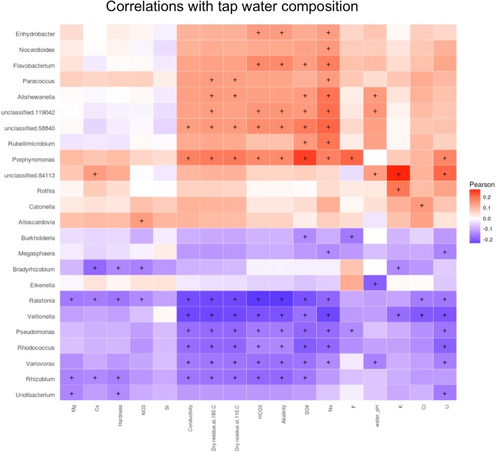
“Porphyromonas was positively associated with the presence of fluoride (F) and sulfate (SO4) in tap water.”
§ Citizen science charts two major “stomatotypes” in the oral microbiome of adolescents and reveals links with habits and drinking water composition > Results > Tap water influences the oral microbiome
plainstates an association- Asserted: passes — The authors put it forward as true.
- Checkable: passes — It can be checked against evidence.
- Load-bearing: passes — The paper’s conclusions depend on it.
- Based: passes — The paper gives a reason why it holds.
- Rests on an assumption: The chemical composition of tap water in the nearest town represents the tap water consumed by participants.
A result the paper reports from its own data — it cites no other source for it, so there is none to check. The quote shows it is in the paper.
In the paper
“In contrast, flossing or using supplemental fluoride mouth wash did not seem to significantly impact the oral microbiome.”
§ Citizen science charts two major “stomatotypes” in the oral microbiome of adolescents and reveals links with habits and drinking water composition > Results > Hygiene habits and saliva pH
hedged- Asserted: passes — The authors put it forward as true.
- Checkable: passes — It can be checked against evidence.
- Load-bearing: unclear — It is unclear whether the paper’s conclusions depend on it.
- Based: passes — The paper gives a reason why it holds.
- Rests on an assumption: Questionnaire responses accurately reflect participants' habits and health.
A result the paper reports from its own data — it cites no other source for it, so there is none to check. The quote shows it is in the paper.
In the paper
“Other genera such as Streptococcus or Veillonella, among others, correlated negatively with saliva pH [see Additional file 7].”
§ Citizen science charts two major “stomatotypes” in the oral microbiome of adolescents and reveals links with habits and drinking water composition > Results > Hygiene habits and saliva pH
plainstates an association- Asserted: passes — The authors put it forward as true.
- Checkable: passes — It can be checked against evidence.
- Load-bearing: unclear — It is unclear whether the paper’s conclusions depend on it.
- Based: passes — The paper gives a reason why it holds.
A result the paper reports from its own data — it cites no other source for it, so there is none to check. The quote shows it is in the paper.
In the paper
“No strong correlation was found between the two stomatotypes and any of the 17 water parameters investigated.”
§ Citizen science charts two major “stomatotypes” in the oral microbiome of adolescents and reveals links with habits and drinking water composition > Results > Tap water influences the oral microbiome
plain- Asserted: passes — The authors put it forward as true.
- Checkable: passes — It can be checked against evidence.
- Load-bearing: passes — The paper’s conclusions depend on it.
- Based: passes — The paper gives a reason why it holds.
- Rests on an assumption: The chemical composition of tap water in the nearest town represents the tap water consumed by participants.
A result the paper reports from its own data — it cites no other source for it, so there is none to check. The quote shows it is in the paper.
In the paper
“We found that living in rural or urban areas did not correlate with significant changes in the microbiome.”
§ Citizen science charts two major “stomatotypes” in the oral microbiome of adolescents and reveals links with habits and drinking water composition > Results > Lifestyle and social parameters
plain- Asserted: passes — The authors put it forward as true.
- Checkable: passes — It can be checked against evidence.
- Load-bearing: unclear — It is unclear whether the paper’s conclusions depend on it.
- Based: passes — The paper gives a reason why it holds.
- Rests on an assumption: Questionnaire responses accurately reflect participants' habits and health.
- It may state two separate claims as one. 57
- Probably not a substantial claim. 40
Every source the paper cites for this claim was checked and supports it.
In the paper
“Similar to previous oral microbiome surveys [7, 29], we found high alpha (within sample) diversity (mean Shannon diversity 2.5, see Additional file 3) and low beta (between samples) diversity (mean weighted UniFrac distance 0.118).”
§ Citizen science charts two major “stomatotypes” in the oral microbiome of adolescents and reveals links with habits and drinking water composition > Results > Oral microbiome diversity is structured into two major stomatotypes
What the sources say
- Supportedcites [7] Moon J-H, Lee J-H. Probing the diversity of healthy oral microbiome with bioinformatics approaches. BMB Rep. 2016;49:662–70. source
The Composition and Diversity of Oral Microbiome section reports high alpha diversity in oral habitats and the lowest beta diversity across subjects compared with other body sites. The citing sentence presents the Shannon and UniFrac means as its authors’ own findings; it cites this paper for the similarity to previous surveys, not for those numerical values. (LLM, conf=0.92)
- Supportedcites [29] Human T, Project M. Structure, function and diversity of the healthy human microbiome. Nature 2012;486:207–214. Available from: http://www.pubmedcentral.nih.gov/articlerender.fcgi?artid=3564958&tool=pmcentrez&rendertype=abstract source
The citation supports the comparison to previous oral microbiome surveys, not the citing authors’ own numerical results introduced by “we found.” In “Microbial diversity of healthy humans,” the source reports that saliva had among the highest alpha diversities and one of the lowest beta diversities. (LLM, conf=0.91)
plain- Asserted: passes — The authors put it forward as true.
- Checkable: passes — It can be checked against evidence.
- Load-bearing: unclear — It is unclear whether the paper’s conclusions depend on it.
- Based: passes — The paper gives a reason why it holds.
It may state two separate claims as one.
- Supported
The sources with a verdict support this claim; the rest weren’t checked yet, have no full text we could read, or their verdicts aren’t rated yet.
In the paper
“An analysis of the oral microbiome in 268 healthy young adults (18–32) classified the samples into five discrete clusters [22], whereas another study of 161 healthy adults found three different clusters [16].”
§ Citizen science charts two major “stomatotypes” in the oral microbiome of adolescents and reveals links with habits and drinking water composition > Results > Oral microbiome diversity is structured into two major stomatotypes
What the sources say
- Not checked yetcites [22] Zaura E, Brandt BW, Prodan A, Teixeira, De Mattos MJ, Imangaliyev S, Kool J, et al. On the ecosystemic network of saliva in healthy young adults. ISME J. 2017;11:1218–31. source
Checked before — its earlier verdict is held back until a new check runs.
- Supportedcites [16] De Filippis F, Vannini L, La Storia A, Laghi L, Piombino P, Stellato G, et al. The same microbiota and a potentially discriminant metabolome in the saliva of omnivore, ovo-lacto-vegetarian and vegan individuals. PLoS One. 2014;9:e112373. source
The Results section reports that PAM analysis of saliva samples identified three salivary types, and its Figure 1 caption gives the sample size as 161. The Discussion states that none of the subjects’ salivary microbiota suggested oral disease. The five-cluster finding is attached to a different citation, not this source. (LLM, conf=0.92)
plain- Asserted: passes — The authors put it forward as true.
- Checkable: passes — It can be checked against evidence.
- Load-bearing: passes — The paper’s conclusions depend on it.
- Based: passes — The paper gives a reason why it holds.
Probably not a substantial claim. It may state two separate claims as one.
- Not checked yet
The cited sources support only part of this claim — read each source’s verdict below.
In the paper
“The core microbiome comprised typical oral bacteria that are commonly identified as abundant in similar oral microbiome surveys [28].”
§ Citizen science charts two major “stomatotypes” in the oral microbiome of adolescents and reveals links with habits and drinking water composition > Discussion
What the sources say
- Partly supportedcites [28] Zaura E, Keijser BJ, Huse SM, Crielaard W. Defining the healthy “core microbiome” of oral microbial communities. BMC Microbiol 2009;9:259. Available from: http://bmcmicrobiol.biomedcentral.com/articles/10.1186/1471-2180-9-259 sourceExperimental — accuracy not yet measured
The Results and Discussion (Sample-specific profiles; Overlap of three individual oral microbiomes, page unavailable) identify taxa present across the three healthy individuals and report that shared higher taxa accounted for 99.8% of reads. The passages do not establish that those particular bacteria were commonly identified as abundant in other oral microbiome surveys. (LLM, conf=0.82)
plain- Asserted: passes — The authors put it forward as true.
- Checkable: passes — It can be checked against evidence.
- Load-bearing: fails — The paper’s conclusions may not depend on it.
- Based: passes — The paper gives a reason why it holds.
Probably not a substantial claim. The paper’s conclusions may not depend on it.
- Partly supported
Every source the paper cites for this claim was checked and supports it.
In the paper
“Previous studies have shown that individual microbiomes from certain niches can be clustered into different types, such as the enterotypes of the gut microbiome [31].”
§ Citizen science charts two major “stomatotypes” in the oral microbiome of adolescents and reveals links with habits and drinking water composition > Results > Oral microbiome diversity is structured into two major stomatotypes
What the sources say
- Supportedcites [31] Arumugam M, Raes J, Pelletier E, Le P, Yamada T, Mende DR, et al. Enterotypes of the human gut microbiome. Nature. 2011;473:174–80. source
In “Robust clustering of samples across nations: Identification of enterotypes,” the paper reports that gut microbiome samples formed three distinct clusters, which it designates enterotypes. This supports the cited example of individual microbiomes from a particular niche being clustered into types; the sentence does not attribute findings about other niches to this paper. (LLM, conf=0.94)
plainstates an association- Asserted: passes — The authors put it forward as true.
- Checkable: passes — It can be checked against evidence.
- Load-bearing: passes — The paper’s conclusions depend on it.
- Based: passes — The paper gives a reason why it holds.
Probably not a substantial claim.
- Supported
The cited sources support only part of this claim — read each source’s verdict below.
In the paper
“Thus, the abundance covariations observed in both stomatotypes may partly reflect the underlying diversity of biofilm succession stages comprised in our samples and would support the main axis of previously observed core community changes in dental plaque.”
§ Citizen science charts two major “stomatotypes” in the oral microbiome of adolescents and reveals links with habits and drinking water composition > Results > Oral microbiome diversity is structured into two major stomatotypes
What the sources say
- Partly supportedcites [1] Kilian M, Chapple ILC, Hannig M, Marsh PD, Meuric V, Pedersen a ML, et al. The oral microbiome – an update for oral healthcare professionals. Bdj. 2016;221:657–66. sourceExperimental — accuracy not yet measured
The section on dysbiosis describes changes in bacterial proportions as dental plaque accumulates, and the discussion of maturing biofilm links maturation to a shift in the microbiota. That supports the general idea that plaque communities change as biofilms develop. Our copy does not identify a main axis of core-community change or connect it to abundance covariations in two stomatotypes; the latter is the citing authors’ interpretation of their samples. (LLM, conf=0.77)
- Not checked — no full text of the sourcecites [32] Jakubovics NS. Intermicrobial interactions as a driver for community composition and stratification of oral biofilms. J Mol Biol. 2015;427:3662–75. source
- Supportedcites [33] Takeshita T, Yasui M, Shibata Y, Furuta M, Saeki Y, Eshima N, et al. Dental plaque development on a hydroxyapatite disk in young adults observed by using a barcoded pyrosequencing approach. Sci Rep 2015;5:8136. Available from: http://www.nature.com/articles/srep08136 source
The Results report that plaque accumulation time significantly affected community composition and that the microbiota shifted over time along principal coordinate 1. The paper also documents changes in bacterial abundances between early and later stages. The sentence’s interpretation of covariations in its own samples is the citing authors’ inference, not a finding attributed to this source. (LLM, conf=0.89)
- Supportedcites [34] Mahajan A, Singh B, Kashyap D, Kumar A, Mahajan P. Interspecies communication and periodontal disease. Sci World J. 2013;2013:765434 source
Section 2, “Biofilms,” describes sequential colonisation of dental plaque and shifts in its microbial composition as the biofilm matures. That supports the cited background point about previously observed community changes; the interpretation of covariations in the citing authors’ stomatotypes is their own. (LLM, conf=0.88)
hedgedstates a possible cause- Asserted: passes — The authors put it forward as true.
- Checkable: passes — It can be checked against evidence.
- Load-bearing: unclear — It is unclear whether the paper’s conclusions depend on it.
- Based: passes — The paper gives a reason why it holds.
It may state two separate claims as one.
- Partly supported
The cited sources support only part of this claim — read each source’s verdict below.
In the paper
“However, earlier studies using similar collection protocols and including information on plaque status or dental health have found correlations between microbial composition of saliva, the amount of plaque and diseases such as periodontitis, or caries [5, 9, 35, 36].”
§ Citizen science charts two major “stomatotypes” in the oral microbiome of adolescents and reveals links with habits and drinking water composition > Results > Oral microbiome diversity is structured into two major stomatotypes
What the sources say
- Partly supportedcites [5] Belstrøm D, Constancias F, Liu Y, Yang L, Drautz-Moses DI, Schuster SC, et al. Metagenomic and metatranscriptomic analysis of saliva reveals disease-associated microbiota in patients with periodontitis and dental caries. NPJ Biofilms Microbiomes 2017;3:23. Available from: http://www.nature.com/articles/s41522-017-0031-4 sourceExperimental — accuracy not yet measured
The Results section ('Salivary abundance of specific oral bacterial species associates with periodontitis and dental caries'; page unavailable) links differences in salivary microbial composition to both diseases. The Methods section ('Study population and sample collection'; page unavailable) describes standardized saliva collection and dental-health classifications, but the paper does not report a correlation with the amount of plaque. (LLM, conf=0.85)
- Supportedcites [9] Takeshita T, Kageyama S, Furuta M, Tsuboi H, Takeuchi K, Shibata Y, et al. Bacterial diversity in saliva and oral health-related conditions: the Hisayama study. Sci Rep. 2016;6:22164. source
The Results (Phylogenetic diversity and oral health-related conditions; page not provided) report significant associations between salivary bacterial diversity and plaque index, decayed teeth, and periodontal-pocket depth. The Methods (Saliva collection and DNA extraction; page not provided) describe the saliva collection protocol, while the dental-examination methods document plaque and dental-health assessments. (LLM, conf=0.90)
- Supportedcites [35] Belstrøm D, Holmstrup P, Fiehn N-E, Kirkby N, Kokaras A, Paster BJ, et al. Salivary microbiota in individuals with different levels of caries experience. J Oral Microbiol Taylor & Francis. 2017;9:1270614. source
The Materials and methods sections describe stimulated-saliva collection and an oral examination recording caries. The Discussion reports an association between salivary bacterial composition and differing levels of caries experience. This supports the caries example for which this paper is cited alongside other studies. (LLM, conf=0.90)
- Supportedcites [36] Zhou J, Jiang N, Wang S, Hu X, Jiao K, He X, et al. Exploration of human salivary microbiomes insights into the novel characteristics of microbial community structure in caries and caries-free subjects. PLoS One. 2016;11:e0147039. source
The Methods (page not specified) describe collecting unstimulated saliva and recording dental health in caries and caries-free subjects. The Results and Discussion (page not specified) report a significant difference in salivary bacterial composition between those groups. In this multi-citation sentence, the paper supports the caries example; it is not being relied on for the plaque-amount or periodontitis examples. (LLM, conf=0.90)
plainstates an association- Asserted: passes — The authors put it forward as true.
- Checkable: passes — It can be checked against evidence.
- Load-bearing: fails — The paper’s conclusions may not depend on it.
- Based: passes — The paper gives a reason why it holds.
Probably not a substantial claim. The paper’s conclusions may not depend on it.
- Partly supported
The cited sources support only part of this claim — read each source’s verdict below.
In the paper
“Most of these genera comprise anaerobic Gram negative species or Gram positives associated to acidic fermentations, which are generally associated to mature biofilm acidification, as well as caries and periodontal disease [3].”
§ Citizen science charts two major “stomatotypes” in the oral microbiome of adolescents and reveals links with habits and drinking water composition > Results > Hygiene habits and saliva pH
What the sources say
- Partly supportedcites [3] Hajishengallis E, Parsaei Y, Klein MI, Koo H. Advances in the microbial etiology and pathogenesis of early childhood caries. Mol Oral Microbiol. 2017;32:24–34. sourceExperimental — accuracy not yet measured
The sections on ECC microbiota and the biofilm matrix describe acid-producing bacteria contributing to plaque acidification and caries. The section on other bacteria also discusses Gram-negative Prevotella in severe ECC plaque. Our copy does not establish that most of the citing paper’s genera have the stated Gram-staining or anaerobic characteristics, or associate them with periodontal disease. (LLM, conf=0.84)
plainstates an association- Asserted: passes — The authors put it forward as true.
- Checkable: passes — It can be checked against evidence.
- Load-bearing: unclear — It is unclear whether the paper’s conclusions depend on it.
- Based: passes — The paper gives a reason why it holds.
It may state two separate claims as one.
- Partly supported
Every source the paper cites for this claim was checked and supports it.
In the paper
“Of note, several of the correlations mentioned in our study coincide with those found in previous studies [16, 22].”
§ Citizen science charts two major “stomatotypes” in the oral microbiome of adolescents and reveals links with habits and drinking water composition > Results > Oral microbiome diversity is structured into two major stomatotypes
What the sources say
- Supportedcites [16] De Filippis F, Vannini L, La Storia A, Laghi L, Piombino P, Stellato G, et al. The same microbiota and a potentially discriminant metabolome in the saliva of omnivore, ovo-lacto-vegetarian and vegan individuals. PLoS One. 2014;9:e112373. source
The Results section (‘OTU co-occurrence and/or co-exclusion’; page unavailable) reports several correlations among salivary bacterial genera. This supports citing the paper as a previous study that found correlations; whether they coincide with the citing authors’ results is the citing authors’ comparison, not a finding attributed to this source. (LLM, conf=0.86)
- Supportedcites [22] Zaura E, Brandt BW, Prodan A, Teixeira, De Mattos MJ, Imangaliyev S, Kool J, et al. On the ecosystemic network of saliva in healthy young adults. ISME J. 2017;11:1218–31. source
The citation points to this paper as a previous study that found correlations; the statement that they coincide with the citing authors’ results is the citing authors’ comparison. The Results sections report correlations among salivary taxa and between microbial taxa and metabolites. The sentence does not specify which correlations overlap, so the overlap itself cannot be checked against this source alone. (LLM, conf=0.88)
plainstates an association- Asserted: passes — The authors put it forward as true.
- Checkable: passes — It can be checked against evidence.
- Load-bearing: fails — The paper’s conclusions may not depend on it.
- Based: passes — The paper gives a reason why it holds.
Probably not a substantial claim. The paper’s conclusions may not depend on it.
- Supported
Every source the paper cites for this claim was checked and supports it.
In the paper
“This study suggested that environment is the main determinant of the oral microbiome with differences between mono- or di-zygotic twins not being significant.”
§ Citizen science charts two major “stomatotypes” in the oral microbiome of adolescents and reveals links with habits and drinking water composition > Background
What the sources say
- Supportedcites [27] Stahringer SS, Clemente JC, Corley RP, Hewitt J, Knights D, Walters WA, et al. Nurture trumps nature in a longitudinal survey of salivary bacterial communities in twins from early adolescence to early adulthood. Genome Res. 2012;22:2146–52. source
The Discussion states that monozygotic twins were somewhat more similar in salivary microbial composition than dizygotic twins, but the difference was not statistically significant. It concludes that environment has a greater impact on overall oral microbiome composition in the studied age range. (LLM, conf=0.94)
hedgedstates a causen = 107- Asserted: fails — The authors may not put it forward as true.
- Checkable: passes — It can be checked against evidence.
- Load-bearing: fails — The paper’s conclusions may not depend on it.
- Based: passes — The paper gives a reason why it holds.
Probably not a substantial claim. The authors may not put it forward as true. The paper’s conclusions may not depend on it. It may state two separate claims as one.
- Supported
The sources with a verdict support this claim; the rest weren’t checked yet, have no full text we could read, or their verdicts aren’t rated yet.
In the paper
“In terms of the driving species, our stomatotypes 1 and 2 are similar, respectively, to MIC1.3 and MIC2 of the 268 adults study and to clusters 1 and 2 of the 161 adults study.”
§ Citizen science charts two major “stomatotypes” in the oral microbiome of adolescents and reveals links with habits and drinking water composition > Results > Oral microbiome diversity is structured into two major stomatotypes
What the sources say
- Supportedcites [16] De Filippis F, Vannini L, La Storia A, Laghi L, Piombino P, Stellato G, et al. The same microbiota and a potentially discriminant metabolome in the saliva of omnivore, ovo-lacto-vegetarian and vegan individuals. PLoS One. 2014;9:e112373. source
The Results (‘The salivary microbiota is not correlated to dietary habit’) identify this as a study of 161 saliva samples and describe the driving genera of clusters I and II: Neisseria and Fusobacterium for cluster I, and Prevotella for cluster II. The citation identifies the 161-person study and its clusters; the comparison with the citing authors’ stomatotypes is their own interpretation. (LLM, conf=0.92)
- Not checked yetcites [22] Zaura E, Brandt BW, Prodan A, Teixeira, De Mattos MJ, Imangaliyev S, Kool J, et al. On the ecosystemic network of saliva in healthy young adults. ISME J. 2017;11:1218–31. source
Checked before — its earlier verdict is held back until a new check runs.
plainstates an association- Asserted: passes — The authors put it forward as true.
- Checkable: passes — It can be checked against evidence.
- Load-bearing: passes — The paper’s conclusions depend on it.
- Based: passes — The paper gives a reason why it holds.
It may state two separate claims as one.
- Supported
Every source the paper cites for this claim was checked and supports it.
In the paper
“These questions were adapted from questionnaires available at the PhenX toolkit (consensus measures for Phenotypes and eXposures), which provides recommended standard data collection protocols for conducting biomedical research [60] and which has been recommended by the microbiome research community [61].”
§ Citizen science charts two major “stomatotypes” in the oral microbiome of adolescents and reveals links with habits and drinking water composition > Material and methods > Questionnaire and other metadata
What the sources say
- Supportedcites [60] Hendershot T, Pan H, Haines J, Harlan WR, Marazita ML, CA MC, et al. Using the PhenX toolkit to add standard measures to a study. Curr Protoc Hum Genet. 2015;86:1.21.1–17. source
The Introduction states that PhenX protocols can be questions for a survey instrument and provide standard procedures for collecting measures in biomedical research. The Key Concepts section also describes the Toolkit’s recommended measures and standard protocols. The separate claim about recommendation by the microbiome research community is attributed to citation [61], not this source. (LLM, conf=0.92)
- Supportedcites [61] Huttenhower C, Knight R, Brown CT, Caporaso JG, Clemente JC, Gevers D, et al. Advancing the microbiome research community. Cell. 2014;159:227–30. source
The citation to this paper [61] supports the statement that the microbiome research community recommends PhenX. In “Assaying and Understanding the Microbiome,” the paper presents PhenX as a model for annotating microbiome metadata and says adherence to its standard would be especially useful. The separate claim about standard data-collection protocols is attributed to [60], not this source. (LLM, conf=0.91)
plain- Asserted: passes — The authors put it forward as true.
- Checkable: passes — It can be checked against evidence.
- Load-bearing: fails — The paper’s conclusions may not depend on it.
- Based: passes — The paper gives a reason why it holds.
Probably not a substantial claim. The paper’s conclusions may not depend on it. It may state two separate claims as one.
- Supported
A result the paper reports from its own data — it cites no other source for it, so there is none to check. The quote shows it is in the paper.
In the paper
“Although 108 students declared smoking occasionally, we did not detect significant differences in their microbiomes.”
§ Citizen science charts two major “stomatotypes” in the oral microbiome of adolescents and reveals links with habits and drinking water composition > Results > Lifestyle and social parameters
plain- Asserted: passes — The authors put it forward as true.
- Checkable: passes — It can be checked against evidence.
- Load-bearing: unclear — It is unclear whether the paper’s conclusions depend on it.
- Based: passes — The paper gives a reason why it holds.
It may state two separate claims as one.
- Rests on an assumption: Questionnaire responses accurately reflect participants' habits and health.
A result the paper reports from its own data — it cites no other source for it, so there is none to check. The quote shows it is in the paper.
In the paper
“The students were more often consuming sweets and chewing gum, while teachers were consuming significantly more coffee and alcohol, reported more dental health problems, and used flossing more frequently.”
§ Citizen science charts two major “stomatotypes” in the oral microbiome of adolescents and reveals links with habits and drinking water composition > Results > Lifestyle and social parameters
plainstates an association- Asserted: passes — The authors put it forward as true.
- Checkable: passes — It can be checked against evidence.
- Load-bearing: unclear — It is unclear whether the paper’s conclusions depend on it.
- Based: passes — The paper gives a reason why it holds.
It may state two separate claims as one.
- Rests on an assumption: Questionnaire responses accurately reflect participants' habits and health.
A result the paper reports from its own data — it cites no other source for it, so there is none to check. The quote shows it is in the paper.
In the paper
“Socioeconomic status did correlate significantly with the abundance of some genera, positively with Rhizobium and negatively with Bradyrhizobium, Acinetobacter, and Pseudomonas.”
§ Citizen science charts two major “stomatotypes” in the oral microbiome of adolescents and reveals links with habits and drinking water composition > Results > Lifestyle and social parameters
plainstates an association- Asserted: passes — The authors put it forward as true.
- Checkable: passes — It can be checked against evidence.
- Load-bearing: unclear — It is unclear whether the paper’s conclusions depend on it.
- Based: passes — The paper gives a reason why it holds.
It may state two separate claims as one.
- Rests on an assumption: Questionnaire responses accurately reflect participants' habits and health.
A result the paper reports from its own data — it cites no other source for it, so there is none to check. The quote shows it is in the paper.
In the paper
“Measured oral pH in our samples had a median of 7.5 but showed a wide range [see Additional file 9].”
§ Citizen science charts two major “stomatotypes” in the oral microbiome of adolescents and reveals links with habits and drinking water composition > Results > Hygiene habits and saliva pH
plain- Asserted: passes — The authors put it forward as true.
- Checkable: passes — It can be checked against evidence.
- Load-bearing: unclear — It is unclear whether the paper’s conclusions depend on it.
- Based: passes — The paper gives a reason why it holds.
It may state two separate claims as one.
A result the paper reports from its own data — it cites no other source for it, so there is none to check. The quote shows it is in the paper.
In the paper
“The top ten most abundant genera represented collectively 84.64% of the analyzed sequences and were present in 99.6% of the samples.”
§ Citizen science charts two major “stomatotypes” in the oral microbiome of adolescents and reveals links with habits and drinking water composition > Results > Oral microbiome diversity is structured into two major stomatotypes
plain- Asserted: passes — The authors put it forward as true.
- Checkable: passes — It can be checked against evidence.
- Load-bearing: unclear — It is unclear whether the paper’s conclusions depend on it.
- Based: passes — The paper gives a reason why it holds.
It may state two separate claims as one.
None of the sources cited for this claim have been checked yet.
In the paper
“For instance, 20 of our 32 common genera are also common in a recent study of the oral microbiome of 2343 adults in Hisayama (Japan) [9].”
§ Citizen science charts two major “stomatotypes” in the oral microbiome of adolescents and reveals links with habits and drinking water composition > Results > Oral microbiome diversity is structured into two major stomatotypes
What the sources say
- Not checked yetcites [9] Takeshita T, Kageyama S, Furuta M, Tsuboi H, Takeuchi K, Shibata Y, et al. Bacterial diversity in saliva and oral health-related conditions: the Hisayama study. Sci Rep. 2016;6:22164. source
Checked before — its earlier verdict is held back until a new check runs.
plain- Asserted: passes — The authors put it forward as true.
- Checkable: passes — It can be checked against evidence.
- Load-bearing: fails — The paper’s conclusions may not depend on it.
- Based: passes — The paper gives a reason why it holds.
Probably not a substantial claim. The paper’s conclusions may not depend on it.
- Not checked yet
A result the paper reports from its own data — it cites no other source for it, so there is none to check. The quote shows it is in the paper.
In the paper
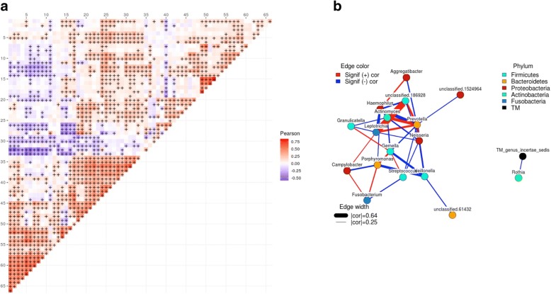
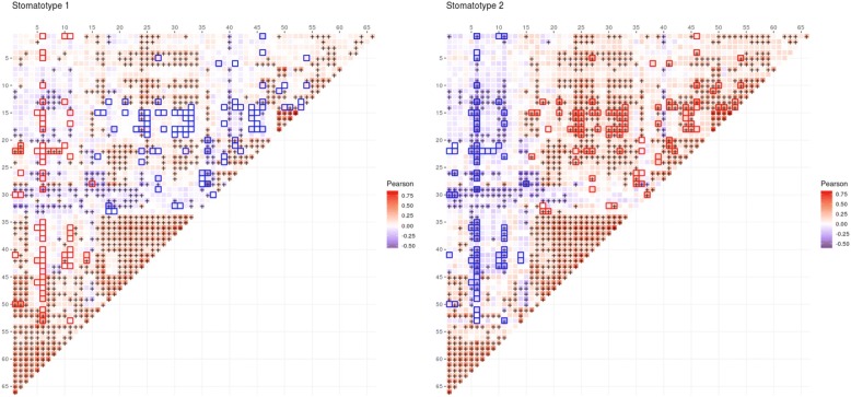
“In both stomatotypes, Streptococcus is positively correlated with Gemella and negatively with Prevotella and Fusobacterium (Fig. 3c).”
§ Citizen science charts two major “stomatotypes” in the oral microbiome of adolescents and reveals links with habits and drinking water composition > Results > Oral microbiome diversity is structured into two major stomatotypes
plainstates an association- Asserted: passes — The authors put it forward as true.
- Checkable: passes — It can be checked against evidence.
- Load-bearing: passes — The paper’s conclusions depend on it.
- Based: passes — The paper gives a reason why it holds.
It may state two separate claims as one.
None of the sources cited for this claim have been checked yet.
In the paper
“These patterns show striking similarities with those found in unrelated populations.”
- Also stated in: § Oral microbiome diversity is structured into two major stomatotypes · boosted
“Importantly, although the studies are performed with different methodologies and have largely different target populations, we noted a strong parallelism between our two stomatotypes and the defined “coinhabiting groups” in the abovementioned Hisayama study [9].”
- Also stated in: § Discussion · plain
“Importantly, our two defined stomatotypes show notable overlap with the two “coinhabiting” groups of bacteria identified in another large study [9].”
§ Citizen science charts two major “stomatotypes” in the oral microbiome of adolescents and reveals links with habits and drinking water composition > Abstract > Results
What the sources say
- Not checked yetcites [9] Takeshita T, Kageyama S, Furuta M, Tsuboi H, Takeuchi K, Shibata Y, et al. Bacterial diversity in saliva and oral health-related conditions: the Hisayama study. Sci Rep. 2016;6:22164. source
Checked before — its earlier verdict is held back until a new check runs.
boostedstates an association- Asserted: passes — The authors put it forward as true.
- Checkable: passes — It can be checked against evidence.
- Load-bearing: passes — The paper’s conclusions depend on it.
- Based: passes — The paper gives a reason why it holds.
It may state two separate claims as one.
- Also stated in: § Oral microbiome diversity is structured into two major stomatotypes · boosted
A result the paper reports from its own data — it cites no other source for it, so there is none to check. The quote shows it is in the paper.
In the paper
“Hygiene habits usually showed high correlations among themselves, so that people who brush their teeth more often tended to use fluoride supplements and floss and were more likely to wash their hands before eating and/or after using the bathroom.”
§ Citizen science charts two major “stomatotypes” in the oral microbiome of adolescents and reveals links with habits and drinking water composition > Results > Hygiene habits and saliva pH
plainstates an association- Asserted: passes — The authors put it forward as true.
- Checkable: passes — It can be checked against evidence.
- Load-bearing: unclear — It is unclear whether the paper’s conclusions depend on it.
- Based: passes — The paper gives a reason why it holds.
It may state two separate claims as one.
- Rests on an assumption: Questionnaire responses accurately reflect participants' habits and health.
The paper states this without a source or data behind it here, so there is nothing to check it against. The quote shows it is in the paper.
In the paper
“All genera discussed in the paper with the exception of Rubellimicrobium and Undibacterium have been previously identified in oral samples.”
§ Citizen science charts two major “stomatotypes” in the oral microbiome of adolescents and reveals links with habits and drinking water composition > Discussion
plain- Asserted: passes — The authors put it forward as true.
- Checkable: passes — It can be checked against evidence.
- Load-bearing: fails — The paper’s conclusions may not depend on it.
- Based: fails — The paper may give no reason why it holds.
Probably not a substantial claim. The paper’s conclusions may not depend on it. The paper may give no reason why it holds.
A result the paper reports from its own data — it cites no other source for it, so there is none to check. The quote shows it is in the paper.
In the paper
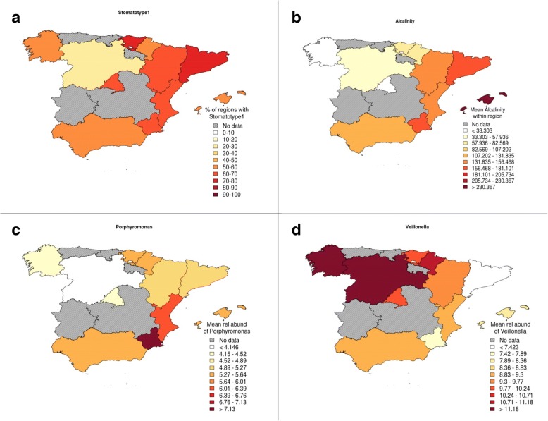
“Notably, however, the two stomatotypes, and some genera, were geographically widespread but showed distinct abundance patterns, which suggest some environmental influence.”
§ Citizen science charts two major “stomatotypes” in the oral microbiome of adolescents and reveals links with habits and drinking water composition > Results > Tap water influences the oral microbiome
hedgedstates an association- Asserted: passes — The authors put it forward as true.
- Checkable: passes — It can be checked against evidence.
- Load-bearing: passes — The paper’s conclusions depend on it.
- Based: passes — The paper gives a reason why it holds.
It may state two separate claims as one.
A result the paper reports from its own data — it cites no other source for it, so there is none to check. The quote shows it is in the paper.
In the paper
“For instance, smokers tend to consume more alcohol, and students who reported having a kissing partner were more likely to smoke, drink alcohol, or chew gum [see Additional file 6].”
§ Citizen science charts two major “stomatotypes” in the oral microbiome of adolescents and reveals links with habits and drinking water composition > Results > Lifestyle and social parameters
plainstates an association- Asserted: passes — The authors put it forward as true.
- Checkable: passes — It can be checked against evidence.
- Load-bearing: fails — The paper’s conclusions may not depend on it.
- Based: passes — The paper gives a reason why it holds.
Probably not a substantial claim. The paper’s conclusions may not depend on it. It may state two separate claims as one.
- Rests on an assumption: Questionnaire responses accurately reflect participants' habits and health.
A result the paper reports from its own data — it cites no other source for it, so there is none to check. The quote shows it is in the paper.
In the paper
“Streptococcus was the most abundant genus in most (68%) samples and showed an average relative abundance of 22.3%, followed by Prevotella (11.9%), Haemophilus (11.4%), Neisseria (10.1%), and Veillonella (9%).”
§ Citizen science charts two major “stomatotypes” in the oral microbiome of adolescents and reveals links with habits and drinking water composition > Results > Oral microbiome diversity is structured into two major stomatotypes
plain- Asserted: passes — The authors put it forward as true.
- Checkable: passes — It can be checked against evidence.
- Load-bearing: unclear — It is unclear whether the paper’s conclusions depend on it.
- Based: passes — The paper gives a reason why it holds.
It may state two separate claims as one.
A result the paper reports from its own data — it cites no other source for it, so there is none to check. The quote shows it is in the paper.
In the paper
“In contrast, we did not find many differences between genders or rural versus urban environment.”
§ Citizen science charts two major “stomatotypes” in the oral microbiome of adolescents and reveals links with habits and drinking water composition > Discussion
plain- Asserted: passes — The authors put it forward as true.
- Checkable: passes — It can be checked against evidence.
- Load-bearing: unclear — It is unclear whether the paper’s conclusions depend on it.
- Based: passes — The paper gives a reason why it holds.
It may state two separate claims as one.
- Rests on an assumption: Questionnaire responses accurately reflect participants' habits and health.
A result the paper reports from its own data — it cites no other source for it, so there is none to check. The quote shows it is in the paper.
In the paper
“We found no large differences between oral microbiomes of males and females, with only two genera (Actinomyces and Oribacterium) showing significantly different abundances (both higher in males).”
§ Citizen science charts two major “stomatotypes” in the oral microbiome of adolescents and reveals links with habits and drinking water composition > Results > Lifestyle and social parameters
plain- Asserted: passes — The authors put it forward as true.
- Checkable: passes — It can be checked against evidence.
- Load-bearing: unclear — It is unclear whether the paper’s conclusions depend on it.
- Based: passes — The paper gives a reason why it holds.
It may state two separate claims as one.
- Rests on an assumption: Questionnaire responses accurately reflect participants' habits and health.
A result the paper reports from its own data — it cites no other source for it, so there is none to check. The quote shows it is in the paper.
In the paper
“Additionally, people using braces were more often brushing their teeth, and those reporting past nerve extractions drank more alcohol.”
§ Citizen science charts two major “stomatotypes” in the oral microbiome of adolescents and reveals links with habits and drinking water composition > Results > Hygiene habits and saliva pH
plainstates an association- Asserted: passes — The authors put it forward as true.
- Checkable: passes — It can be checked against evidence.
- Load-bearing: unclear — It is unclear whether the paper’s conclusions depend on it.
- Based: passes — The paper gives a reason why it holds.
It may state two separate claims as one.
- Rests on an assumption: Questionnaire responses accurately reflect participants' habits and health.
A result the paper reports from its own data — it cites no other source for it, so there is none to check. The quote shows it is in the paper.
In the paper
“Other differences include higher proportions of Haemophilus in stomatotype 1 and higher proportions of Veillonella and Streptococcus in stomatotype 2.”
§ Citizen science charts two major “stomatotypes” in the oral microbiome of adolescents and reveals links with habits and drinking water composition > Results > Oral microbiome diversity is structured into two major stomatotypes
plainstates an association- Asserted: passes — The authors put it forward as true.
- Checkable: passes — It can be checked against evidence.
- Load-bearing: unclear — It is unclear whether the paper’s conclusions depend on it.
- Based: passes — The paper gives a reason why it holds.
It may state two separate claims as one.
A result the paper reports from its own data — it cites no other source for it, so there is none to check. The quote shows it is in the paper.
In the paper
“Interestingly, students with kissing partners had a higher number of taxa in their microbiomes, which also showed a significantly higher presence of Treponema.”
§ Citizen science charts two major “stomatotypes” in the oral microbiome of adolescents and reveals links with habits and drinking water composition > Results > Lifestyle and social parameters
plainstates an association- Asserted: passes — The authors put it forward as true.
- Checkable: passes — It can be checked against evidence.
- Load-bearing: unclear — It is unclear whether the paper’s conclusions depend on it.
- Based: passes — The paper gives a reason why it holds.
It may state two separate claims as one.
- Rests on an assumption: Questionnaire responses accurately reflect participants' habits and health.
A result the paper reports from its own data — it cites no other source for it, so there is none to check. The quote shows it is in the paper.
In the paper
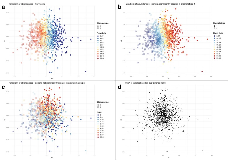
“The stomatotypes are driven mostly by certain abundant genera, but do not explain the variability found in many other genera.”
§ Citizen science charts two major “stomatotypes” in the oral microbiome of adolescents and reveals links with habits and drinking water composition > Results > Oral microbiome diversity is structured into two major stomatotypes
plainstates a cause- Asserted: passes — The authors put it forward as true.
- Checkable: passes — It can be checked against evidence.
- Load-bearing: unclear — It is unclear whether the paper’s conclusions depend on it.
- Based: passes — The paper gives a reason why it holds.
It may state two separate claims as one.
A result the paper reports from its own data — it cites no other source for it, so there is none to check. The quote shows it is in the paper.
In the paper
“Although many of the covariations between the two stomatotypes are similar, their strengths can be markedly different. In addition, some covariations appear specific for each stomatotype.”
§ Citizen science charts two major “stomatotypes” in the oral microbiome of adolescents and reveals links with habits and drinking water composition > Results > Oral microbiome diversity is structured into two major stomatotypes
hedgedstates an association- Asserted: passes — The authors put it forward as true.
- Checkable: passes — It can be checked against evidence.
- Load-bearing: passes — The paper’s conclusions depend on it.
- Based: passes — The paper gives a reason why it holds.
It may state two separate claims as one.
A result the paper reports from its own data — it cites no other source for it, so there is none to check. The quote shows it is in the paper.
In the paper
“Overall, we identified 332 operational taxonomic units (OTUs) at the genus level in our dataset.”
§ Citizen science charts two major “stomatotypes” in the oral microbiome of adolescents and reveals links with habits and drinking water composition > Results > Oral microbiome diversity is structured into two major stomatotypes
plain- Asserted: passes — The authors put it forward as true.
- Checkable: passes — It can be checked against evidence.
- Load-bearing: fails — The paper’s conclusions may not depend on it.
- Based: passes — The paper gives a reason why it holds.
Probably not a substantial claim. The paper’s conclusions may not depend on it.
A result the paper reports from its own data — it cites no other source for it, so there is none to check. The quote shows it is in the paper.
In the paper
“Ralstonia abundance was also negatively affected by nearly all other water variables, and it was the genus whose abundance changed the most with tap water quality, followed by Rhizobium, Veillonella, and Pseudomonas.”
§ Citizen science charts two major “stomatotypes” in the oral microbiome of adolescents and reveals links with habits and drinking water composition > Results > Tap water influences the oral microbiome
plainstates a cause- Asserted: passes — The authors put it forward as true.
- Checkable: passes — It can be checked against evidence.
- Load-bearing: passes — The paper’s conclusions depend on it.
- Based: passes — The paper gives a reason why it holds.
It may state two separate claims as one.
- Rests on an assumption: The chemical composition of tap water in the nearest town represents the tap water consumed by participants.
A result the paper reports from its own data — it cites no other source for it, so there is none to check. The quote shows it is in the paper.
In the paper
“Boys and girls had some different habits. While the former tended to drink more milk, coke, or energetic drinks, the latter chewed gum and brushed their teeth more often.”
§ Citizen science charts two major “stomatotypes” in the oral microbiome of adolescents and reveals links with habits and drinking water composition > Results > Lifestyle and social parameters
plainstates an association- Asserted: passes — The authors put it forward as true.
- Checkable: passes — It can be checked against evidence.
- Load-bearing: unclear — It is unclear whether the paper’s conclusions depend on it.
- Based: passes — The paper gives a reason why it holds.
It may state two separate claims as one.
- Rests on an assumption: Questionnaire responses accurately reflect participants' habits and health.
A result the paper reports from its own data — it cites no other source for it, so there is none to check. The quote shows it is in the paper.
In the paper
“Overall, the microbiome samples of our study can be clustered into two broad compositional patterns (stomatotypes), driven mostly by Neisseria and Prevotella, respectively.”
- Also stated in: § Oral microbiome diversity is structured into two major stomatotypes · plain
“The two defined stomatotypes differ in their microbial composition and abundance covariations, and for which Neisseria (stomatotype 1) and Prevotella (stomatotype 2) are the genera driving most differences (Fig. 3).”
- Also stated in: § Discussion · plain
“We found that the oral microbiome of the studied population can be broadly classified into two different stomatotypes.”
§ Citizen science charts two major “stomatotypes” in the oral microbiome of adolescents and reveals links with habits and drinking water composition > Abstract > Results
plainstates a cause- Asserted: passes — The authors put it forward as true.
- Checkable: passes — It can be checked against evidence.
- Load-bearing: passes — The paper’s conclusions depend on it.
- Based: passes — The paper gives a reason why it holds.
It may state two separate claims as one.
- Also stated in: § Oral microbiome diversity is structured into two major stomatotypes · plain
None of the sources cited for this claim have been checked yet.
In the paper
“Yet, many parallels can also be found between our stomatotypes, and those in these studies.”
- Also stated in: § Discussion · boosted
“Although other studies have defined higher number of clusters in the oral microbiome [16, 22], some of these clusters show clear similarities with the two stomatotypes found in this study.”
§ Citizen science charts two major “stomatotypes” in the oral microbiome of adolescents and reveals links with habits and drinking water composition > Results > Oral microbiome diversity is structured into two major stomatotypes
What the sources say
- Not checked yetcites [16] De Filippis F, Vannini L, La Storia A, Laghi L, Piombino P, Stellato G, et al. The same microbiota and a potentially discriminant metabolome in the saliva of omnivore, ovo-lacto-vegetarian and vegan individuals. PLoS One. 2014;9:e112373. source
- Not checked yetcites [22] Zaura E, Brandt BW, Prodan A, Teixeira, De Mattos MJ, Imangaliyev S, Kool J, et al. On the ecosystemic network of saliva in healthy young adults. ISME J. 2017;11:1218–31. source
Checked before — its earlier verdict is held back until a new check runs.
boostedstates an association- Asserted: passes — The authors put it forward as true.
- Checkable: passes — It can be checked against evidence.
- Load-bearing: passes — The paper’s conclusions depend on it.
- Based: passes — The paper gives a reason why it holds.
It may state two separate claims as one.
- Also stated in: § Discussion · boosted
The paper states this without a source or data behind it here, so there is nothing to check it against. The quote shows it is in the paper.
In the paper
“The core oral microbiome described in this study is composed of genera commonly identified in other oral microbiome studies.”
§ Citizen science charts two major “stomatotypes” in the oral microbiome of adolescents and reveals links with habits and drinking water composition > Conclusions
plain- Asserted: passes — The authors put it forward as true.
- Checkable: passes — It can be checked against evidence.
- Load-bearing: fails — The paper’s conclusions may not depend on it.
- Based: passes — The paper gives a reason why it holds.
Probably not a substantial claim. The paper’s conclusions may not depend on it.
A result the paper reports from its own data — it cites no other source for it, so there is none to check. The quote shows it is in the paper.
In the paper
“However, the two stomatotypes do contain a significant amount of variability and a gradient of variation, sometimes unrelated to the stomatotypes, is observed for the most abundant genera.”
§ Citizen science charts two major “stomatotypes” in the oral microbiome of adolescents and reveals links with habits and drinking water composition > Discussion
plain- Asserted: passes — The authors put it forward as true.
- Checkable: passes — It can be checked against evidence.
- Load-bearing: unclear — It is unclear whether the paper’s conclusions depend on it.
- Based: passes — The paper gives a reason why it holds.
It may state two separate claims as one.
A result the paper reports from its own data — it cites no other source for it, so there is none to check. The quote shows it is in the paper.
In the paper
“Three hundred thirty-two different genera were identified in these samples.”
§ Citizen science charts two major “stomatotypes” in the oral microbiome of adolescents and reveals links with habits and drinking water composition > Material and methods > Microbiome composition profiling
plainn = 1,319- Asserted: passes — The authors put it forward as true.
- Checkable: passes — It can be checked against evidence.
- Load-bearing: fails — The paper’s conclusions may not depend on it.
- Based: passes — The paper gives a reason why it holds.
Probably not a substantial claim. The paper’s conclusions may not depend on it.
A result the paper reports from its own data — it cites no other source for it, so there is none to check. The quote shows it is in the paper.
In the paper
“Although the presence of the most abundant genera of the oral microbiome such as Streptococcus, Prevotella, or Haemophilus (the top three in our samples) were not significantly affected by tap water, some genera among the ten most abundant were affected, including Veillonella, Porphyromonas, and Gemella.”
§ Citizen science charts two major “stomatotypes” in the oral microbiome of adolescents and reveals links with habits and drinking water composition > Discussion
plain- Asserted: passes — The authors put it forward as true.
- Checkable: passes — It can be checked against evidence.
- Load-bearing: passes — The paper’s conclusions depend on it.
- Based: passes — The paper gives a reason why it holds.
It may state two separate claims as one.
- Rests on an assumption: The chemical composition of tap water in the nearest town represents the tap water consumed by participants.
None of the sources cited for this claim have been checked yet.
In the paper
“The two studies coincide in defining higher proportions of Neisseria, Haemophilus, and Porphyromonas, in one of the types (stomatotype 1, coinhabiting group 2), and those of Prevotella, and Veillonella in the other (stomatotype 2, coinhabiting group 1).”
§ Citizen science charts two major “stomatotypes” in the oral microbiome of adolescents and reveals links with habits and drinking water composition > Discussion
What the sources say
- Not checked yetcites [9] Takeshita T, Kageyama S, Furuta M, Tsuboi H, Takeuchi K, Shibata Y, et al. Bacterial diversity in saliva and oral health-related conditions: the Hisayama study. Sci Rep. 2016;6:22164. source
Checked before — its earlier verdict is held back until a new check runs.
plainstates an association- Asserted: passes — The authors put it forward as true.
- Checkable: passes — It can be checked against evidence.
- Load-bearing: passes — The paper’s conclusions depend on it.
- Based: passes — The paper gives a reason why it holds.
It may state two separate claims as one.
- Not checked yet
What the paper did — it cites no source for this, so there is none to check. The quote shows it is in the paper.
In the paper
“However, we cannot discard the possibility that some of the low abundance genera identified are not stable components of the oral cavity but result from sporadic colonization from the close environment of the donor (i.e., food, air, or water).”
§ Citizen science charts two major “stomatotypes” in the oral microbiome of adolescents and reveals links with habits and drinking water composition > Discussion
hedgedstates a possible cause- Asserted: passes — The authors put it forward as true.
- Checkable: passes — It can be checked against evidence.
- Load-bearing: fails — The paper’s conclusions may not depend on it.
- Based: passes — The paper gives a reason why it holds.
Probably not a substantial claim. The paper’s conclusions may not depend on it.
None of the sources cited for this claim have been checked yet.
In the paper
“For instance, in the case of stomatotype 1, we detected positive covariation of Fusobacterium and Capnocytophaga, both anaerobic bacteria implicated in dental plaque progression [33], while in stomatotype 2, we specifically detect antagonism between Streptococcus and Actinomyces, which are known to compete in the initial phases of dental plaque formation [32, 37].”
§ Citizen science charts two major “stomatotypes” in the oral microbiome of adolescents and reveals links with habits and drinking water composition > Results > Oral microbiome diversity is structured into two major stomatotypes
What the sources say
- Not checked yetcites [33] Takeshita T, Yasui M, Shibata Y, Furuta M, Saeki Y, Eshima N, et al. Dental plaque development on a hydroxyapatite disk in young adults observed by using a barcoded pyrosequencing approach. Sci Rep 2015;5:8136. Available from: http://www.nature.com/articles/srep08136 source
Checked before — its earlier verdict is held back until a new check runs.
plainstates an association- Asserted: passes — The authors put it forward as true.
- Checkable: passes — It can be checked against evidence.
- Load-bearing: fails — The paper’s conclusions may not depend on it.
- Based: passes — The paper gives a reason why it holds.
Probably not a substantial claim. The paper’s conclusions may not depend on it.
- Not checked yet
A conclusion the paper draws from its own results — it cites no other source for it, so there is none to check. The quote shows it is in the paper.
In the paper
“Some of these differences may relate to the fact that some habits, such as smoking or some dietary habits, may have just been recently established, or the habit is more sporadic in adolescents, and the effects in the microbiome will only be apparent after a prolonged period of sustained habit.”
§ Citizen science charts two major “stomatotypes” in the oral microbiome of adolescents and reveals links with habits and drinking water composition > Discussion
hedgedstates a possible cause- Asserted: passes — The authors put it forward as true.
- Checkable: passes — It can be checked against evidence.
- Load-bearing: fails — The paper’s conclusions may not depend on it.
- Based: fails — The paper may give no reason why it holds.
Probably not a substantial claim. The paper’s conclusions may not depend on it. The paper may give no reason why it holds. It may state two separate claims as one.
A conclusion the paper draws from its own results — it cites no other source for it, so there is none to check. The quote shows it is in the paper.
In the paper
“Positive correlations between Porphyromonas and Fusobacterium and negative correlations between Veillonella and Gemella further support this model, while positive correlations between Porphyromonas and Gemella and negative correlations between Porphyromonas and Veillonella would not be explained by the current plaque succession model.”
§ Citizen science charts two major “stomatotypes” in the oral microbiome of adolescents and reveals links with habits and drinking water composition > Results > Oral microbiome diversity is structured into two major stomatotypes
hedgedstates an association- Asserted: passes — The authors put it forward as true.
- Checkable: passes — It can be checked against evidence.
- Load-bearing: passes — The paper’s conclusions depend on it.
- Based: passes — The paper gives a reason why it holds.
It may state two separate claims as one.
What the paper did — it cites no source for this, so there is none to check. The quote shows it is in the paper.
In the paper
“Microbial compositions in oral rinse samples can only be considered a proxy for plaque communities, as the procedure collects cells from different oral niches.”
§ Citizen science charts two major “stomatotypes” in the oral microbiome of adolescents and reveals links with habits and drinking water composition > Results > Oral microbiome diversity is structured into two major stomatotypes
plain- Asserted: passes — The authors put it forward as true.
- Checkable: passes — It can be checked against evidence.
- Load-bearing: fails — The paper’s conclusions may not depend on it.
- Based: passes — The paper gives a reason why it holds.
Probably not a substantial claim. The paper’s conclusions may not depend on it.
What the paper did — it cites no source for this, so there is none to check. The quote shows it is in the paper.
In the paper
“In accordance with this, all of our negative controls provided no measurable results and a negligible number of reads when forced into library preparation and sequencing (see the “Materials and samples” section).”
§ Citizen science charts two major “stomatotypes” in the oral microbiome of adolescents and reveals links with habits and drinking water composition > Discussion
plain- Asserted: passes — The authors put it forward as true.
- Checkable: passes — It can be checked against evidence.
- Load-bearing: passes — The paper’s conclusions depend on it.
- Based: passes — The paper gives a reason why it holds.
It may state two separate claims as one.
A conclusion the paper draws from its own results — it cites no other source for it, so there is none to check. The quote shows it is in the paper.
In the paper
“These striking similarities between disparate studies suggest that these two major stomatotypes may be ubiquitous and define global equilibria in the human mouth microbiome.”
- Also stated in: § Discussion · hedged
“That the two disparate studies agree in the two broadly defined groups strongly suggests that these two stomatotypes define two possible equilibria of oral microbial communities which are globally present.”
§ Citizen science charts two major “stomatotypes” in the oral microbiome of adolescents and reveals links with habits and drinking water composition > Results > Oral microbiome diversity is structured into two major stomatotypes
hedged- Asserted: passes — The authors put it forward as true.
- Checkable: passes — It can be checked against evidence.
- Load-bearing: passes — The paper’s conclusions depend on it.
- Based: passes — The paper gives a reason why it holds.
It may state two separate claims as one.
- Also stated in: § Discussion · hedged
In the paper
“It is known that caries is generally associated with an increase of Streptococcus, but also of Granulicatella, and Gemella [21]—although in the latter case, this varies with age [39]—supporting the effect of brushing against primary dental plaque.”
§ Citizen science charts two major “stomatotypes” in the oral microbiome of adolescents and reveals links with habits and drinking water composition > Results > Hygiene habits and saliva pH
What the sources say
- Not checked yetcites [21] Costalonga M, Herzberg MC. The oral microbiome and the immunobiology of periodontal disease and caries. Immunol Lett. 2014;162:22–38. source
boostedstates an association- Asserted: passes — The authors put it forward as true.
- Checkable: passes — It can be checked against evidence.
- Load-bearing: fails — The paper’s conclusions may not depend on it.
- Based: passes — The paper gives a reason why it holds.
Probably not a substantial claim. The paper’s conclusions may not depend on it.
A claim is checked only against the cited paper’s full text, never its abstract, and none is available for its sources.
In the paper
“For instance, in the case of stomatotype 1, we detected positive covariation of Fusobacterium and Capnocytophaga, both anaerobic bacteria implicated in dental plaque progression [33], while in stomatotype 2, we specifically detect antagonism between Streptococcus and Actinomyces, which are known to compete in the initial phases of dental plaque formation [32, 37].”
§ Citizen science charts two major “stomatotypes” in the oral microbiome of adolescents and reveals links with habits and drinking water composition > Results > Oral microbiome diversity is structured into two major stomatotypes
What the sources say
- Not checked — no full text of the sourcecites [32] Jakubovics NS. Intermicrobial interactions as a driver for community composition and stratification of oral biofilms. J Mol Biol. 2015;427:3662–75. source
- Not checked — no full text of the sourcecites [37] Dige I, Raarup MK, Nyengaard JR, Kilian M, Nyvad B. Actinomyces naeslundii in initial dental biofilm formation. Microbiology. 2009;155:2116–26. source
boostedstates an association- Asserted: passes — The authors put it forward as true.
- Checkable: passes — It can be checked against evidence.
- Load-bearing: fails — The paper’s conclusions may not depend on it.
- Based: passes — The paper gives a reason why it holds.
Probably not a substantial claim. The paper’s conclusions may not depend on it.
A conclusion the paper draws from its own results — it cites no other source for it, so there is none to check. The quote shows it is in the paper.
In the paper
“For instance, strong co-occurrence links Leptotrichia, Actinomyces, and Prevotella, and this latter one with Veillonella, suggesting they may be ecologically related.”
§ Citizen science charts two major “stomatotypes” in the oral microbiome of adolescents and reveals links with habits and drinking water composition > Results > Oral microbiome diversity is structured into two major stomatotypes
hedgedstates an association- Asserted: passes — The authors put it forward as true.
- Checkable: passes — It can be checked against evidence.
- Load-bearing: unclear — It is unclear whether the paper’s conclusions depend on it.
- Based: passes — The paper gives a reason why it holds.
It may state two separate claims as one.
In the paper
“Veillonella species are known to increase their abundance in acidic environments derived from fermentation processes, such as those occurring in mature dental plaque [3].”
§ Citizen science charts two major “stomatotypes” in the oral microbiome of adolescents and reveals links with habits and drinking water composition > Results > Hygiene habits and saliva pH
What the sources say
- Not checked yetcites [3] Hajishengallis E, Parsaei Y, Klein MI, Koo H. Advances in the microbial etiology and pathogenesis of early childhood caries. Mol Oral Microbiol. 2017;32:24–34. source
boostedstates a cause- Asserted: passes — The authors put it forward as true.
- Checkable: passes — It can be checked against evidence.
- Load-bearing: fails — The paper’s conclusions may not depend on it.
- Based: passes — The paper gives a reason why it holds.
Probably not a substantial claim. The paper’s conclusions may not depend on it.
A conclusion the paper draws from its own results — it cites no other source for it, so there is none to check. The quote shows it is in the paper.
In the paper
“Adolescence is a stage with major hormonal and habit changes, which likely impact the oral microbial community.”
§ Citizen science charts two major “stomatotypes” in the oral microbiome of adolescents and reveals links with habits and drinking water composition > Discussion
hedgedstates a possible cause- Asserted: passes — The authors put it forward as true.
- Checkable: passes — It can be checked against evidence.
- Load-bearing: fails — The paper’s conclusions may not depend on it.
- Based: fails — The paper may give no reason why it holds.
Probably not a substantial claim. The paper’s conclusions may not depend on it. The paper may give no reason why it holds. It may state two separate claims as one.
None of the sources cited for this claim have been checked yet.
In the paper
“It is known that caries is generally associated with an increase of Streptococcus, but also of Granulicatella, and Gemella [21]—although in the latter case, this varies with age [39]—supporting the effect of brushing against primary dental plaque.”
§ Citizen science charts two major “stomatotypes” in the oral microbiome of adolescents and reveals links with habits and drinking water composition > Results > Hygiene habits and saliva pH
What the sources say
- Not checked yetcites [39] Holgerson PL, Öhman C, Rönnlund A, Johansson I. Maturation of oral microbiota in children with or without dental caries. PLoS One. 2015;10:e0128534. source
Checked before — its earlier verdict is held back until a new check runs.
plainstates an association- Asserted: passes — The authors put it forward as true.
- Checkable: passes — It can be checked against evidence.
- Load-bearing: fails — The paper’s conclusions may not depend on it.
- Based: passes — The paper gives a reason why it holds.
Probably not a substantial claim. The paper’s conclusions may not depend on it.
- Not checked yet
None of the sources cited for this claim have been checked yet.
In the paper
“Selenomonas has been described as one of the most abundant taxa during orthodontic braces treatment and has been linked to common oral diseases such as gingivitis [19].”
§ Citizen science charts two major “stomatotypes” in the oral microbiome of adolescents and reveals links with habits and drinking water composition > Results > Hygiene habits and saliva pH
What the sources say
- Not checked yetcites [19] Koopman JE, van der Kaaij NCW, Buijs MJ, Elyassi Y, van der Veen MH, Crielaard W, et al. The effect of fixed orthodontic appliances and fluoride mouthwash on the oral microbiome of adolescents - a randomized controlled clinical trial. PLoS One 2015;10:e0137318. Available from: http://www.ncbi.nlm.nih.gov/pubmed/26332408%5Cn http://www.pubmedcentral.nih.gov/articlerender.fcgi?artid=PMC4558009 source
Checked before — its earlier verdict is held back until a new check runs.
plainstates an association- Asserted: passes — The authors put it forward as true.
- Checkable: passes — It can be checked against evidence.
- Load-bearing: fails — The paper’s conclusions may not depend on it.
- Based: passes — The paper gives a reason why it holds.
Probably not a substantial claim. The paper’s conclusions may not depend on it. It may state two separate claims as one.
- Not checked yet
A conclusion the paper draws from its own results — it cites no other source for it, so there is none to check. The quote shows it is in the paper.
In the paper
“The patterns were sometimes reminiscent of maps of certain public water quality parameters, such as alkalinity or water hardness, which differ significantly across regions in Spain (Fig. 6).”
§ Citizen science charts two major “stomatotypes” in the oral microbiome of adolescents and reveals links with habits and drinking water composition > Results > Tap water influences the oral microbiome
hedgedstates an association- Asserted: passes — The authors put it forward as true.
- Checkable: passes — It can be checked against evidence.
- Load-bearing: passes — The paper’s conclusions depend on it.
- Based: passes — The paper gives a reason why it holds.
It may state two separate claims as one.
A conclusion the paper draws from its own results — it cites no other source for it, so there is none to check. The quote shows it is in the paper.
In the paper
“In addition, the oral microbiome of adolescents may have specificities as a transition phase from childhood to adulthood.”
§ Citizen science charts two major “stomatotypes” in the oral microbiome of adolescents and reveals links with habits and drinking water composition > Discussion
hedgedstates a possible cause- Asserted: passes — The authors put it forward as true.
- Checkable: passes — It can be checked against evidence.
- Load-bearing: fails — The paper’s conclusions may not depend on it.
- Based: passes — The paper gives a reason why it holds.
Probably not a substantial claim. The paper’s conclusions may not depend on it.
What the paper did — it cites no source for this, so there is none to check. The quote shows it is in the paper.
In the paper
“Admittedly, measurements of saliva pH using pH strips—a limitation imposed in part by our citizen science approach—lack the precision provided by a pH meter (see “Materials and methods” section).”
§ Citizen science charts two major “stomatotypes” in the oral microbiome of adolescents and reveals links with habits and drinking water composition > Results > Hygiene habits and saliva pH
plain- Asserted: passes — The authors put it forward as true.
- Checkable: passes — It can be checked against evidence.
- Load-bearing: fails — The paper’s conclusions may not depend on it.
- Based: passes — The paper gives a reason why it holds.
Probably not a substantial claim. The paper’s conclusions may not depend on it.
In the paper
“Higher oral pH was positively correlated with the abundance of Fusobacterium and Porphyromonas, a bacterial genus known to grow optimally in alkaline environments, and able to increase the pH of its medium [38].”
§ Citizen science charts two major “stomatotypes” in the oral microbiome of adolescents and reveals links with habits and drinking water composition > Results > Hygiene habits and saliva pH
What the sources say
- Not checked — no full text of the sourcecites [38] Takahashi N, Schachtele CF. Effect of pH on the growth and proteolytic activity of Porphyromonas gingivalis and Bacteroides intermedius. J Dent Res. 1990;69:1266–9. source
boostedstates a cause- Asserted: passes — The authors put it forward as true.
- Checkable: passes — It can be checked against evidence.
- Load-bearing: fails — The paper’s conclusions may not depend on it.
- Based: passes — The paper gives a reason why it holds.
Probably not a substantial claim. The paper’s conclusions may not depend on it. It may state two separate claims as one.
In the paper
“In fact, this period of life is associated with a sharp increase in the incidence and severity of gingivitis [45], which may be related to underlying oral microbiome changes.”
§ Citizen science charts two major “stomatotypes” in the oral microbiome of adolescents and reveals links with habits and drinking water composition > Discussion
What the sources say
- Not checked — no full text of the sourcecites [45] Mombelli A, Gusberti FA, van Oosten MAC, Lang NP. Gingival health and gingivitis development during puberty: a 4-year longitudinal study. J Clin Periodontol. 1989;16:451–6. source
plainstates an association- Asserted: passes — The authors put it forward as true.
- Checkable: passes — It can be checked against evidence.
- Load-bearing: fails — The paper’s conclusions may not depend on it.
- Based: passes — The paper gives a reason why it holds.
Probably not a substantial claim. The paper’s conclusions may not depend on it.
None of the sources cited for this claim have been checked yet.
In the paper
“Interestingly, some variables such as body mass index, which is generally associated to alterations in the gut microbiome, and it has been associated to changes in the oral microbiome in adults [44], seemed to have a minor impact on the mouth microbiome of adolescents in our sample.”
§ Citizen science charts two major “stomatotypes” in the oral microbiome of adolescents and reveals links with habits and drinking water composition > Discussion
What the sources say
- Not checked yetcites [44] Shillitoe E, Weinstock R, Kim T, Simon H, Planer J, Noonan S, et al. The oral microflora in obesity and type-2 diabetes. J Oral Microbiol 2012;4:19013. Available from: https://www.tandfonline.com/doi/full/10.3402/jom.v4i0.19013 source
Checked before — its earlier verdict is held back until a new check runs.
plainstates an association- Asserted: passes — The authors put it forward as true.
- Checkable: passes — It can be checked against evidence.
- Load-bearing: fails — The paper’s conclusions may not depend on it.
- Based: passes — The paper gives a reason why it holds.
Probably not a substantial claim. The paper’s conclusions may not depend on it. It may state two separate claims as one.
- Not checked yet
A conclusion the paper draws from its own results — it cites no other source for it, so there is none to check. The quote shows it is in the paper.
In the paper
“These results suggest that tap water composition may be an important, poorly studied factor shaping the oral microbiome.”
- Also stated in: § Results · plain
“This points to an important role of drinking water in shaping the oral microbiota, which has been so far poorly explored.”
§ Citizen science charts two major “stomatotypes” in the oral microbiome of adolescents and reveals links with habits and drinking water composition > Results > Tap water influences the oral microbiome
plainstates a possible cause- Asserted: passes — The authors put it forward as true.
- Checkable: passes — It can be checked against evidence.
- Load-bearing: passes — The paper’s conclusions depend on it.
- Based: passes — The paper gives a reason why it holds.
It may state two separate claims as one.
- Rests on an assumption: The chemical composition of tap water in the nearest town represents the tap water consumed by participants.
- Also stated in: § Results · plain
A conclusion the paper draws from its own results — it cites no other source for it, so there is none to check. The quote shows it is in the paper.
In the paper
“These large differences may be related to age but also to their understandably different lifestyle.”
§ Citizen science charts two major “stomatotypes” in the oral microbiome of adolescents and reveals links with habits and drinking water composition > Results > Lifestyle and social parameters
hedgedstates a possible cause- Asserted: passes — The authors put it forward as true.
- Checkable: passes — It can be checked against evidence.
- Load-bearing: fails — The paper’s conclusions may not depend on it.
- Based: passes — The paper gives a reason why it holds.
Probably not a substantial claim. The paper’s conclusions may not depend on it. It may state two separate claims as one.
A conclusion the paper draws from its own results — it cites no other source for it, so there is none to check. The quote shows it is in the paper.
In the paper
“As we discuss below, these stomatotypes are not discrete, well separated entities, but rather represent two poles of a gradient of microbial compositions.”
§ Citizen science charts two major “stomatotypes” in the oral microbiome of adolescents and reveals links with habits and drinking water composition > Results > Oral microbiome diversity is structured into two major stomatotypes
plain- Asserted: passes — The authors put it forward as true.
- Checkable: passes — It can be checked against evidence.
- Load-bearing: passes — The paper’s conclusions depend on it.
- Based: passes — The paper gives a reason why it holds.
It may state two separate claims as one.
A conclusion the paper draws from its own results — it cites no other source for it, so there is none to check. The quote shows it is in the paper.
In the paper
“Our results thus raise the question of the role of drinking water in shaping the oral microbiome, suggesting a potentially important role.”
§ Citizen science charts two major “stomatotypes” in the oral microbiome of adolescents and reveals links with habits and drinking water composition > Discussion
hedgedstates a possible cause- Asserted: passes — The authors put it forward as true.
- Checkable: passes — It can be checked against evidence.
- Load-bearing: passes — The paper’s conclusions depend on it.
- Based: passes — The paper gives a reason why it holds.
Probably not a substantial claim. It may state two separate claims as one.
- Rests on an assumption: The chemical composition of tap water in the nearest town represents the tap water consumed by participants.
In the paper
“Next, we used the Calinski-Harabasz (CH) index [59] to determine the optimal number of clusters, and we further verified this by calculating the average silhouette width of the samples, which is a measure of the separation of samples within one cluster from those of another cluster, as well as the prediction strength, another measure of the efficiency of clustering.”
§ Citizen science charts two major “stomatotypes” in the oral microbiome of adolescents and reveals links with habits and drinking water composition > Material and methods > Sample clustering
What the sources say
- Not checked — no full text of the sourcecites [59] Calinski T, Harabasz J. A dendrite method for cluster analysis. Commun Stat - Theory Methods. 1974;3:1–27. source
plain- Asserted: passes — The authors put it forward as true.
- Checkable: passes — It can be checked against evidence.
- Load-bearing: passes — The paper’s conclusions depend on it.
- Based: passes — The paper gives a reason why it holds.
Probably not a substantial claim. It may state two separate claims as one.
A conclusion the paper draws from its own results — it cites no other source for it, so there is none to check. The quote shows it is in the paper.
In the paper
“In fact, this period of life is associated with a sharp increase in the incidence and severity of gingivitis [45], which may be related to underlying oral microbiome changes.”
§ Citizen science charts two major “stomatotypes” in the oral microbiome of adolescents and reveals links with habits and drinking water composition > Discussion
hedgedstates a possible cause- Asserted: passes — The authors put it forward as true.
- Checkable: passes — It can be checked against evidence.
- Load-bearing: fails — The paper’s conclusions may not depend on it.
- Based: passes — The paper gives a reason why it holds.
Probably not a substantial claim. The paper’s conclusions may not depend on it.
What the paper did — it cites no source for this, so there is none to check. The quote shows it is in the paper.
In the paper
“Furthemore, the adonis function in the vegan package was used to perform a PERMANOVA test on each beta diversity measure to ensure significant separation of stomatotypes.”
§ Citizen science charts two major “stomatotypes” in the oral microbiome of adolescents and reveals links with habits and drinking water composition > Material and methods > Sample clustering
plainstates an association- Asserted: passes — The authors put it forward as true.
- Checkable: passes — It can be checked against evidence.
- Load-bearing: passes — The paper’s conclusions depend on it.
- Based: passes — The paper gives a reason why it holds.
Probably not a substantial claim.
What the paper did — it cites no source for this, so there is none to check. The quote shows it is in the paper.
In the paper
“As a control for downstream procedures, we also used two DNA samples derived from bacterial mock communities obtained from the BEI Resources of the Human Microbiome Project: Each sample contained genomic DNA of ribosomal operons from 20 bacterial species.”
§ Citizen science charts two major “stomatotypes” in the oral microbiome of adolescents and reveals links with habits and drinking water composition > Material and methods > DNA extraction and sequencing
plainn = 2- Asserted: passes — The authors put it forward as true.
- Checkable: passes — It can be checked against evidence.
- Load-bearing: fails — The paper’s conclusions may not depend on it.
- Based: passes — The paper gives a reason why it holds.
Probably not a substantial claim. The paper’s conclusions may not depend on it.
None of the sources cited for this claim have been checked yet.
In the paper
“Saliva samples were collected using a mouth wash and using a protocol that had been previously tested and compared with other procedures during a pilot phase of the project. Of note, this procedure is used in other oral microbiome studies and have been shown to produce consistent results with other sampling procedures [51].”
§ Citizen science charts two major “stomatotypes” in the oral microbiome of adolescents and reveals links with habits and drinking water composition > Material and methods > Sample collection
What the sources say
- Not checked yetcites [51] Lim Y, Totsika M, Morrison M, Punyadeera C. The saliva microbiome profiles are minimally affected by collection method or DNA extraction protocols. Sci Rep. 2017;7:8523. source
Checked before — its earlier verdict is held back until a new check runs.
plain- Asserted: passes — The authors put it forward as true.
- Checkable: passes — It can be checked against evidence.
- Load-bearing: unclear — It is unclear whether the paper’s conclusions depend on it.
- Based: passes — The paper gives a reason why it holds.
It may state two separate claims as one.
- Not checked yet
What the paper did — it cites no source for this, so there is none to check. The quote shows it is in the paper.
In the paper
“Negative controls of the sample collection buffer, DNA extraction, and PCR amplification steps were routinely performed in parallel, using the same conditions and reagents. Our controls systematically provided no visible band or quantifiable DNA amounts by gel visualization or Bioanalyzer, whereas all of our samples provided clearly visible bands after 20 cycles.”
- Also stated in: § DNA extraction and sequencing · plain
“Four such controls were subjected to library preparation and sequenced. Expectedly, these sequenced non-template controls systematically yielded very few reads (a range of 30–880 reads per sample), in contrast to an average of 54,000 reads/library in sample-derived libraries.”
§ Citizen science charts two major “stomatotypes” in the oral microbiome of adolescents and reveals links with habits and drinking water composition > Material and methods > DNA extraction and sequencing
plainn = 4- Asserted: passes — The authors put it forward as true.
- Checkable: passes — It can be checked against evidence.
- Load-bearing: unclear — It is unclear whether the paper’s conclusions depend on it.
- Based: passes — The paper gives a reason why it holds.
It may state two separate claims as one.
- Also stated in: § DNA extraction and sequencing · plain
In the paper
“Although the use of pH test strips have been validated extensively [50], we validated our chosen strips.”
- Also stated in: § Sample collection · plain
“The correlation was high (R2 = 0.96), with average absolute differences between the value of the pH meter and that provided by the researcher being 0.33 which is within the range of the limit of detection of the method (0.5).”
§ Citizen science charts two major “stomatotypes” in the oral microbiome of adolescents and reveals links with habits and drinking water composition > Material and methods > Sample collection
What the sources say
- Not checked — no full text of the sourcecites [50] Cocco F, Cagetti MG, Lingstrom P, Camoni N, Campus G. The strip method and the microelectrode technique in assessing dental plaque pH. Minerva Stomatol. 2017;66:241–247. source
boostedstates an association- Asserted: passes — The authors put it forward as true.
- Checkable: passes — It can be checked against evidence.
- Load-bearing: unclear — It is unclear whether the paper’s conclusions depend on it.
- Based: passes — The paper gives a reason why it holds.
It may state two separate claims as one.
- Also stated in: § Sample collection · plain
None of the sources cited for this claim have been checked yet.
In the paper
“In this regard, experiments in mice have shown that the composition of tap water can be related with changes in the gut microbiome [47] and have an incidence in the progression of diseases such as diabetes [48].”
§ Citizen science charts two major “stomatotypes” in the oral microbiome of adolescents and reveals links with habits and drinking water composition > Discussion
What the sources say
- Not checked — no full text of the sourcecites [47] Dias MF, Reis MP, Acurcio LB, Carmo AO, Diamantino CF, Motta AM, et al. Changes in mouse gut bacterial community in response to different types of drinking water. Water Res. 2018;132:79–89. source
- Not checked yetcites [48] Wolf KJ, Daft JG, Tanner SM, Hartmann R, Khafipour E, Lorenz RG. Consumption of acidic water alters the gut microbiome and decreases the risk of diabetes in NOD mice. J Histochem Cytochem. 2014;62:237–50. source
Checked before — its earlier verdict is held back until a new check runs.
plainstates an association- Asserted: passes — The authors put it forward as true.
- Checkable: passes — It can be checked against evidence.
- Load-bearing: fails — The paper’s conclusions may not depend on it.
- Based: passes — The paper gives a reason why it holds.
Probably not a substantial claim. The paper’s conclusions may not depend on it. It may state two separate claims as one.
What the paper did — it cites no source for this, so there is none to check. The quote shows it is in the paper.
In the paper
“Clustering was validated using all five distance measures to ensure proper clustering, but analyses here are performed using the clustering based on JSD.”
§ Citizen science charts two major “stomatotypes” in the oral microbiome of adolescents and reveals links with habits and drinking water composition > Material and methods > Sample clustering
plain- Asserted: passes — The authors put it forward as true.
- Checkable: passes — It can be checked against evidence.
- Load-bearing: fails — The paper’s conclusions may not depend on it.
- Based: passes — The paper gives a reason why it holds.
Probably not a substantial claim. The paper’s conclusions may not depend on it. It may state two separate claims as one.
A conclusion the paper draws from its own results — it cites no other source for it, so there is none to check. The quote shows it is in the paper.
In the paper
“the described stomatotypes are common and globally distributed does not preclude the possibility that further, clearly distinct, stomatotypes may be found in other populations.”
§ Citizen science charts two major “stomatotypes” in the oral microbiome of adolescents and reveals links with habits and drinking water composition > Discussion
hedged- Asserted: passes — The authors put it forward as true.
- Checkable: passes — It can be checked against evidence.
- Load-bearing: passes — The paper’s conclusions depend on it.
- Based: unclear — It is unclear why the paper says it holds.
It may state two separate claims as one.
What the paper did — it cites no source for this, so there is none to check. The quote shows it is in the paper.
In the paper
“One hundred eighty samples from 5 of the schools had to be removed due to an apparent batch effect during the sequencing procedure. This batch effect was detected in the initial quality assessment of the comparison of the data.”
- Also stated in: § Microbiome composition profiling · plain
“Additionally, 33 samples were removed from the analyses because of errors with the sample identifiers, leaving a total of 1319 samples from 35 different schools from around Spain.”
§ Citizen science charts two major “stomatotypes” in the oral microbiome of adolescents and reveals links with habits and drinking water composition > Material and methods > Microbiome composition profiling
plainn = 1,319- Asserted: passes — The authors put it forward as true.
- Checkable: passes — It can be checked against evidence.
- Load-bearing: fails — The paper’s conclusions may not depend on it.
- Based: passes — The paper gives a reason why it holds.
Probably not a substantial claim. The paper’s conclusions may not depend on it. It may state two separate claims as one.
- Also stated in: § Microbiome composition profiling · plain
A conclusion the paper draws from its own results — it cites no other source for it, so there is none to check. The quote shows it is in the paper.
In the paper
“This points to an important role of tap water in shaping the oral microbiome, which has been overlooked in previous studies.”
§ Citizen science charts two major “stomatotypes” in the oral microbiome of adolescents and reveals links with habits and drinking water composition > Conclusions
plainstates a cause- Asserted: passes — The authors put it forward as true.
- Checkable: passes — It can be checked against evidence.
- Load-bearing: passes — The paper’s conclusions depend on it.
- Based: passes — The paper gives a reason why it holds.
It may state two separate claims as one.
- Rests on an assumption: The ionic composition of tap water from donors' hometowns, as obtained from national studies, reflects the tap water actually consumed by the donors.
What the paper did — it cites no source for this, so there is none to check. The quote shows it is in the paper.
In the paper
“All participants, and at least one of their parents or legal guardians for those under the age of 18, signed a consent form to use their saliva samples for microbiome research. This consent form and the purpose of this project received approval by the ethics committee of the Barcelona Biomedical Research Park (PRBB).”
§ Citizen science charts two major “stomatotypes” in the oral microbiome of adolescents and reveals links with habits and drinking water composition > Material and methods > Sample collection
plain- Asserted: passes — The authors put it forward as true.
- Checkable: passes — It can be checked against evidence.
- Load-bearing: fails — The paper’s conclusions may not depend on it.
- Based: passes — The paper gives a reason why it holds.
Probably not a substantial claim. The paper’s conclusions may not depend on it. It may state two separate claims as one.
None of the sources cited for this claim have been checked yet.
In the paper
“Previous studies have analyzed the relationship between the presence of fluoride and the incidence of caries [46], but the overall impact on the human oral microbiota of this and other factors remain unexplored.”
§ Citizen science charts two major “stomatotypes” in the oral microbiome of adolescents and reveals links with habits and drinking water composition > Discussion
What the sources say
- Not checked yetcites [46] Iheozor-Ejiofor Z, Worthington H V, Walsh T, O’Malley L, Clarkson JE, Macey R, et al. Water fluoridation for the prevention of dental caries. Cochrane Database Syst Rev. 2015. https://doi.org/10.1002/14651858.CD010856.pub2 . source
Checked before — its earlier verdict is held back until a new check runs.
plain- Asserted: passes — The authors put it forward as true.
- Checkable: passes — It can be checked against evidence.
- Load-bearing: passes — The paper’s conclusions depend on it.
- Based: passes — The paper gives a reason why it holds.
Probably not a substantial claim. It may state two separate claims as one.
- Not checked yet
What the paper did — it cites no source for this, so there is none to check. The quote shows it is in the paper.
In the paper
“The specific pipeline and parameters were set using sequence reads from both 16S rRNA amplicon and whole genome sequencing of the described mock communities.”
§ Citizen science charts two major “stomatotypes” in the oral microbiome of adolescents and reveals links with habits and drinking water composition > Material and methods > Pre-processing of 16S rRNA sequence reads and operational taxonomic unit assignment
plain- Asserted: passes — The authors put it forward as true.
- Checkable: passes — It can be checked against evidence.
- Load-bearing: fails — The paper’s conclusions may not depend on it.
- Based: passes — The paper gives a reason why it holds.
Probably not a substantial claim. The paper’s conclusions may not depend on it.
The paper relies on this without support.
Questionnaire responses accurately reflect participants' habits and health.
“Donors were asked to answer a questionnaire, including 54 questions [see Additional file 2], some of which proposed by citizens, about their health, and their dietary and hygiene habits.”
The paper relies on this without support.
The chemical composition of tap water in the nearest town represents the tap water consumed by participants.
“Hence, we decided to investigate this factor in more detail and linked our samples to the chemical composition of tap water of the nearest town, as reported in recent studies [40–42].”
The paper relies on this without support.
The ionic composition of tap water from donors' hometowns, as obtained from national studies, reflects the tap water actually consumed by the donors.
“Data on tap water hardness was obtained from several national ionic composition studies [40–42].”
The paper relies on this without support.
The questionnaire responses accurately reflect participants' diet and hygiene habits.
“Participants were asked to answer one questionnaire inquiring about aspects relevant to their hygiene and dietary habits. These questions were adapted from questionnaires available at the PhenX toolkit (consensus measures for Phenotypes and eXposures), which provides recommended standard data collection protocols for conducting biomedical research [60] and which has been recommended by the microbi”
Claims other papers make about this one
Each is checked against this paper’s own text: does it say what the citing paper says it does?
In the citing paper
“For example, research by Willis et al. indicated a strong correlation between the composition of tap water and the prevalence of specific bacterial species [11], highlighting the significant impact of drinking water on the oral microbiota.”
From Severity-dependent alterations in oral microbiota and antibiotic resistance in children with dental fluorosis (2026) · cites this paper as [11]
In the citing paper
“Willis et al. further demonstrated that long-term fluoride exposure in adolescents is associated with distinct oral microbial profiles and environmental influences such as drinking water [11].”
From Severity-dependent alterations in oral microbiota and antibiotic resistance in children with dental fluorosis (2026) · cites this paper as [11]
Self-check
Percentages, sums and reported differences re-computed from the paper’s own numbers.
Each contradiction between two passages listed here was confirmed by an independent check.
Rated minor: it would not touch a result — a value no result rests on, a p-value that stays on the same side of the significance level, or a conflict that is clerical, resolved elsewhere in the paper, or outside its own findings.
In the paper
§ Citizen science charts two major “stomatotypes” in the oral microbiome of adolescents and reveals links with habits and drinking water composition > Results > Oral microbiome diversity is structured into two major stomatotypes
“this figure shows only the 67 genera which were present in at least 1/3 of all samples (436).”
§ Citizen science charts two major “stomatotypes” in the oral microbiome of adolescents and reveals links with habits and drinking water composition > Material and methods > Microbiome composition profiling
“leaving a total of 1319 samples from 35 different schools from around Spain.”
Rated minor: it would not touch a result — a value no result rests on, a p-value that stays on the same side of the significance level, or a conflict that is clerical, resolved elsewhere in the paper, or outside its own findings.
In the paper
§ Citizen science charts two major “stomatotypes” in the oral microbiome of adolescents and reveals links with habits and drinking water composition > Results > Oral microbiome diversity is structured into two major stomatotypes
“Edges indicate significant positive (red) or negative (blue) correlations between indicated genera. Edge width is proportional to Pearson correlation coefficient. Only displaying edges for coefficients of 0.25 or greater.”
§ Citizen science charts two major “stomatotypes” in the oral microbiome of adolescents and reveals links with habits and drinking water composition > Material and methods > Co-occurrence networks
“edges are formed between only those genera that have a correlation coefficient greater than 0.25 or less than − 0.25 and an adjusted p value less than 0.05.”
Citations
Cites
vegan: Community Ecology Package
Oksanen, J., Simpson, G. L., Blanchet, F. G., Kindt, R., Legendre, P., Minchin, P. R., O’Hara, R. B., Sólymos, P., Stevens, M. H. H., Szöcs, E., et al. (2001) · doi:10.32614/cran.package.vegan · Cited by 27,099
phyloseq: An R Package for Reproducible Interactive Analysis and Graphics of Microbiome Census Data
McMurdie, P. J., & Holmes, S. (2013) · PLoS ONE · doi:10.1371/journal.pone.0061217 · Cited by 21,942
Schloss, P. D., Westcott, S. L., Ryabin, T., Hall, J. R., Hartmann, M., Hollister, E. B., Lesniewski, R. A., Oakley, B. B., Parks, D. H., Robinson, C. J., et al. (2009) · Applied and Environmental Microbiology · doi:10.1128/aem.01541-09 · Cited by 19,549
Structure, function and diversity of the healthy human microbiome
The Human Microbiome Project Consortium (2012) · Nature · doi:10.1038/nature11234 · Cited by 11,726
Enterotypes of the human gut microbiome
MetaHIT Consortium (additional members), Arumugam, M., Raes, J., Pelletier, E., Le Paslier, D., Yamada, T., Mende, D. R., Fernandes, G. R., Tap, J., Bruls, T., et al. (2011) · Nature · doi:10.1038/nature09944 · Cited by 7,548
Pruesse, E., Quast, C., Knittel, K., Fuchs, B. M., Ludwig, W., Peplies, J., & Glöckner, F. O. (2007) · Nucleic Acids Research · doi:10.1093/nar/gkm864 · Cited by 6,786
A dendrite method for cluster analysis
Caliński, T., & Harabasz, J. (1974) · Communications in Statistics · doi:10.1080/03610927408827101 · Cited by 4,480
Reagent and laboratory contamination can critically impact sequence-based microbiome analyses
Salter, S. J., Cox, M. J., Turek, E. M., Calus, S. T., Cookson, W. O., Moffatt, M. F., Turner, P., Parkhill, J., Loman, N. J., & Walker, A. W. (2014) · BMC Biology · doi:10.1186/s12915-014-0087-z · Cited by 3,463
Occlusal Caries: Biological Approach for Its Diagnosis and Management
Carvalho, J. C., Dige, I., Mačhiulskienė, V., Qvist, V., Bakhshandeh, A., Parolo, C. C. F., & Maltz, M. (2016) · Caries Research · doi:10.1159/000448662 · Cited by 2,159
The oral microbiome in health and disease
Wade, W. G. (2013) · Pharmacological Research · doi:10.1016/j.phrs.2012.11.006 · Cited by 1,347
Defining the healthy “core microbiome” of oral microbial communities
Zaura, E., Keijser, B. J., Huse, S. M., & Crielaard, W. (2009) · BMC Microbiology · doi:10.1186/1471-2180-9-259 · Cited by 1,323
The oral microbiome – an update for oral healthcare professionals
Kilian, M., Chapple, I. L. C., Hannig, M., Marsh, P. D., Meuric, V., Pedersen, A. M. L., Tonetti, M. S., Wade, W. G., & Zaura, E. (2016) · British Dental Journal · doi:10.1038/sj.bdj.2016.865 · Cited by 1,269 · cited 3×
“In addition, given the close connections of the oral cavity with the vascular system and the digestive and respiratory tracks, alterations of the mouth microbiota have been related with diseases that affect other body parts, such as diabetes or cardiovascular disease [1, 4].”
BackgroundMorris, E. K., Caruso, T., Buscot, F., Fischer, M., Hancock, C., Maier, T. S., Meiners, T., Müller, C., Obermaier, E., Prati, D., et al. (2014) · Ecology and Evolution · doi:10.1002/ece3.1155 · Cited by 1,258
Bioconductor Workflow for Microbiome Data Analysis: from raw reads to community analyses
Callahan, B. J., Sankaran, K., Fukuyama, J., McMurdie, P. J., & Holmes, S. (2016) · F1000Research · doi:10.12688/f1000research.8986.2 · Cited by 1,148
The oral microbiome and the immunobiology of periodontal disease and caries
Costalonga, M., & Herzberg, M. C. (2014) · Immunology Letters · doi:10.1016/j.imlet.2014.08.017 · Cited by 645
Cigarette smoking and the oral microbiome in a large study of American adults
Wu, J., Peters, B. A., Dominianni, C., Zhang, Y., Pei, Z., Yang, L., Ma, Y., Purdue, M. P., Jacobs, E. J., Gapstur, S. M., et al. (2016) · The ISME Journal · doi:10.1038/ismej.2016.37 · Cited by 572 · cited 1×
“[11, 12], diet [13–16], or hygiene habits [17–19].”
Saliva in the diagnosis of diseases
Zhang, C.-Z., Cheng, X., Li, J., Zhang, P., Yi, P., Xu, X., & Zhou, X. (2016) · International Journal of Oral Science · doi:10.1038/ijos.2016.38 · Cited by 570
Knights, D., Ward, T. L., McKinlay, C. E., Miller, H., Gonzalez, A., McDonald, D., & Knight, R. (2014) · Cell Host & Microbe · doi:10.1016/j.chom.2014.09.013 · Cited by 396
Bioconductor workflow for microbiome data analysis: from raw reads to community analyses
Callahan, B. J., Sankaran, K., Fukuyama, J. A., McMurdie, P. J., & Holmes, S. P. (2016) · F1000Research · doi:10.12688/f1000research.8986.1 · Cited by 331
Chen, H., & Jiang, W. (2014) · Frontiers in Microbiology · doi:10.3389/fmicb.2014.00508 · Cited by 317
The oral microbiome diversity and its relation to human diseases
He, J., Li, Y., Cao, Y., Xue, J., & Zhou, X. (2015) · Folia Microbiologica · doi:10.1007/s12223-014-0342-2 · Cited by 314
The oral microbiome and human health
Yamashita, Y., & Takeshita, T. (2017) · Journal of Oral Science · doi:10.2334/josnusd.16-0856 · Cited by 305
Bacterial diversity in saliva and oral health-related conditions: the Hisayama Study
Takeshita, T., Kageyama, S., Furuta, M., Tsuboi, H., Takeuchi, K., Shibata, Y., Shimazaki, Y., Akifusa, S., Ninomiya, T., Kiyohara, Y., et al. (2016) · Scientific Reports · doi:10.1038/srep22164 · Cited by 284
Advances in the microbial etiology and pathogenesis of early childhood caries
Hajishengallis, E., Parsaei, Y., Klein, M. I., & Koo, H. (2017) · Molecular Oral Microbiology · doi:10.1111/omi.12152 · Cited by 261
Water fluoridation for the prevention of dental caries
Iheozor-Ejiofor, Z., Worthington, H. V., Walsh, T., O'Malley, L., Clarkson, J. E., Macey, R., Alam, R., Tugwell, P., Welch, V., & Glenny, A.-M. (2015) · Cochrane Database of Systematic Reviews · doi:10.1002/14651858.cd010856.pub2 · Cited by 214
Microbiomes of Site-Specific Dental Plaques from Children with Different Caries Status
Richards, V. P., Alvarez, A. J., Luce, A. R., Bedenbaugh, M., Mitchell, M. L., Burne, R. A., & Nascimento, M. M. (2017) · Infection and Immunity · doi:10.1128/iai.00106-17 · Cited by 208
The effect of cigarette smoking on the oral and nasal microbiota
Yu, G., Phillips, S., Gail, M. H., Goedert, J. J., Humphrys, M. S., Ravel, J., Ren, Y., & Caporaso, N. E. (2017) · Microbiome · doi:10.1186/s40168-016-0226-6 · Cited by 191
Stahringer, S. S., Clemente, J. C., Corley, R. P., Hewitt, J., Knights, D., Walters, W. A., Knight, R., & Krauter, K. S. (2012) · Genome Research · doi:10.1101/gr.140608.112 · Cited by 180
De Filippis, F., Vannini, L., La Storia, A., Laghi, L., Piombino, P., Stellato, G., Serrazanetti, D. I., Gozzi, G., Turroni, S., Ferrocino, I., et al. (2014) · PLoS ONE · doi:10.1371/journal.pone.0112373 · Cited by 146
On the ecosystemic network of saliva in healthy young adults
Zaura, E., Brandt, B. W., Prodan, A., Teixeira de Mattos, M. J., Imangaliyev, S., Kool, J., Buijs, M. J., Jagers, F. L. P. W., Hennequin-Hoenderdos, N. L., Slot, D. E., et al. (2017) · The ISME Journal · doi:10.1038/ismej.2016.199 · Cited by 142
Belstrøm, D., Constancias, F., Liu, Y., Yang, L., Drautz-Moses, D. I., Schuster, S. C., Kohli, G. S., Jakobsen, T. H., Holmstrup, P., & Givskov, M. (2017) · npj Biofilms and Microbiomes · doi:10.1038/s41522-017-0031-4 · Cited by 125
Lim, Y., Totsika, M., Morrison, M., & Punyadeera, C. (2017) · Scientific Reports · doi:10.1038/s41598-017-07885-3 · Cited by 119
Characterization of oral and gut microbiome temporal variability in hospitalized cancer patients
Galloway-Peña, J., Smith, D. P., Sahasrabhojane, P. V., Wadsworth, W. D., Fellman, B. M., Ajami, N. J., Shpall, E. J., Daver, N. G., Guindani, M., Petrosino, J. F., et al. (2017) · Genome Medicine · doi:10.1186/s13073-017-0409-1 · Cited by 118
Actinomyces naeslundii in initial dental biofilm formation
Dige, I., Raarup, M. K., Nyengaard, J. R., Kilian, M., & Nyvad, B. (2009) · Microbiology · doi:10.1099/mic.0.027706-0 · Cited by 115
Advancements toward a systems level understanding of the human oral microbiome
McLean, J. S. (2014) · Frontiers in Cellular and Infection Microbiology · doi:10.3389/fcimb.2014.00098 · Cited by 108
Jakubovics, N. S. (2015) · Journal of Molecular Biology · doi:10.1016/j.jmb.2015.09.022 · Cited by 107
Maturation of Oral Microbiota in Children with or without Dental Caries
Lif Holgerson, P., Öhman, C., Rönnlund, A., & Johansson, I. (2015) · PLOS ONE · doi:10.1371/journal.pone.0128534 · Cited by 97
Saliva: A diagnostic biomarker of periodontal diseases
Patil, P., & Patil, B. (2011) · Journal of Indian Society of Periodontology · doi:10.4103/0972-124x.92560 · Cited by 97
Kageyama, S., Takeshita, T., Asakawa, M., Shibata, Y., Takeuchi, K., Yamanaka, W., & Yamashita, Y. (2017) · PLoS ONE · doi:10.1371/journal.pone.0174782 · Cited by 95
Distinct composition of the oral indigenous microbiota in South Korean and Japanese adults
Takeshita, T., Matsuo, K., Furuta, M., Shibata, Y., Fukami, K., Shimazaki, Y., Akifusa, S., Han, D.-H., Kim, H., Yokoyama, T., et al. (2014) · Scientific Reports · doi:10.1038/srep06990 · Cited by 83
Takahashi, N., & Schachtele, C. F. (1990) · Journal of Dental Research · doi:10.1177/00220345900690060801 · Cited by 83
Jose, J. E., Padmanabhan, S., & Chitharanjan, A. B. (2013) · American Journal of Orthodontics and Dentofacial Orthopedics · doi:10.1016/j.ajodo.2013.02.023 · Cited by 78
Consumption of Acidic Water Alters the Gut Microbiome and Decreases the Risk of Diabetes in NOD Mice
Wolf, K. J., Daft, J. G., Tanner, S. M., Hartmann, R., Khafipour, E., & Lorenz, R. G. (2014) · Journal of Histochemistry & Cytochemistry · doi:10.1369/0022155413519650 · Cited by 76
Koopman, J. E., van der Kaaij, N. C. W., Buijs, M. J., Elyassi, Y., van der Veen, M. H., Crielaard, W., ten Cate, J. M., & Zaura, E. (2015) · PLOS ONE · doi:10.1371/journal.pone.0137318 · Cited by 74
The role of the commensal microbiota in the regulation of tolerance to dietary allergens
Canani, R. B., Gilbert, J. A., & Nagler‐Anderson, C. (2015) · Current Opinion in Allergy and Clinical Immunology · doi:10.1097/aci.0000000000000157 · Cited by 63
Takeshita, T., Yasui, M., Shibata, Y., Furuta, M., Saeki, Y., Eshima, N., & Yamashita, Y. (2015) · Scientific Reports · doi:10.1038/srep08136 · Cited by 58
Advancing the Microbiome Research Community
Huttenhower, C., Knight, R., Brown, C. T., Caporaso, J. G., Clemente, J. C., Gevers, D., Franzosa, E. A., Kelley, S. T., Knights, D., Ley, R. E., et al. (2014) · Cell · doi:10.1016/j.cell.2014.09.022 · Cited by 58
Gingival health and gingivitis development during puberty: A 4‐year longitudinal study
Mombelli, A., Gusberti, F. A., van Oosten, M. A. C., & Lang, N. P. (1989) · Journal of Clinical Periodontology · doi:10.1111/j.1600-051x.1989.tb01674.x · Cited by 57
Salivary microbiota in individuals with different levels of caries experience
Belstrøm, D., Holmstrup, P., Fiehn, N.-E., Kirkby, N., Kokaras, A., Paster, B. J., & Bardow, A. (2017) · Journal of Oral Microbiology · doi:10.1080/20002297.2016.1270614 · Cited by 54
Probing the diversity of healthy oral microbiome with bioinformatics approaches
Moon, J.-H., & Lee, J.-H. (2016) · BMB Reports · doi:10.5483/bmbrep.2016.49.12.164 · Cited by 53
Klaus, K., Eichenauer, J., Sprenger, R., & Ruf, S. (2016) · Head & Face Medicine · doi:10.1186/s13005-016-0125-x · Cited by 43
Changes in mouse gut bacterial community in response to different types of drinking water
Dias, M. F., Reis, M. P., Acurcio, L. B., Carmo, A. O., Diamantino, C. F., Motta, A. M., Kalapothakis, E., Nicoli, J. R., & Nascimento, A. M. A. (2018) · Water Research · doi:10.1016/j.watres.2017.12.052 · Cited by 43
Zhou, J., Jiang, N., Wang, S., Hu, X., Jiao, K., He, X., Li, Z., & Wang, J. (2016) · PLOS ONE · doi:10.1371/journal.pone.0147039 · Cited by 41
The oral microflora in obesity and type-2 diabetes
Shillitoe, E., Weinstock, R., Kim, T., Simon, H., Planer, J., Noonan, S., & Cooney, R. (2012) · Journal of Oral Microbiology · doi:10.3402/jom.v4i0.19013 · Cited by 38
Cuervo, A., Hevia, A., López, P., Suárez, A., Diaz, C., Sánchez, B., Margolles, A., & González, S. (2016) · Food & Function · doi:10.1039/c5fo00853k · Cited by 32
Al-Mulla, A., Karlsson, L., Kharsa, S. A., Kjellberg, H., & Birkhed, D. (2010) · Acta Odontologica Scandinavica · doi:10.3109/00016357.2010.512863 · Cited by 29
Interspecies Communication and Periodontal Disease
Mahajan, A., Singh, B., Kashyap, D., Kumar, A., & Mahajan, P. (2013) · The Scientific World Journal · doi:10.1155/2013/765434 · Cited by 26
Using the PhenX Toolkit to Add Standard Measures to a Study
Hendershot, T., Pan, H., Haines, J., Harlan, W. R., Marazita, M. L., McCarty, C. A., Ramos, E. M., & Hamilton, C. M. (2015) · Current Protocols in Human Genetics · doi:10.1002/0471142905.hg0121s86 · Cited by 25
Maraver, F., Vitoria, I., Ferreira‐Pêgo, C., Castro, F. A., & Salas‐Salvadó, J. (2015) · PubMed · doi:10.3305/nh.2015.31.5.8589 · Cited by 23
Contenido en nitratos de aguas de consumo público españolas
Vitoria, I., Maraver, F., Sánchez‐Valverde, F., & Castro, F. A. (2015) · Gaceta Sanitaria · doi:10.1016/j.gaceta.2014.12.007 · Cited by 18
Fluoruro en aguas minerales naturales envasadas en España y prevención de la caries dental
Maraver, F., Vitoria, I., Almerich‐Silla, J. M., & Castro, F. A. (2014) · Atención Primaria · doi:10.1016/j.aprim.2014.04.003 · Cited by 16
The strip method and the microelectrode technique in assessing dental plaque pH
Cocco, F., Cagetti, M. G., Lingström, P., Camoni, N., & Campus, G. (2017) · Minerva Dental and Oral Science · doi:10.23736/s0026-4970.17.04093-6 · Cited by 1
Research works printed but not linked: 1
- Maraver F, Vitoria Miñana I, Ferreira-Pêgo C, Armijo F, Salas-Salvadó J. Magnesio en el agua de consume público y aguas minerales naturals en España y su contribución en cubrir las necesidades nutricionales. Nutr Hosp. 2015;31:2297–312.
Cited by
Sorted by citations
Prevotella Diversity, Niches and Interactions with the Human Host
Tett, A., Pasolli, E., Masetti, G., Ercolini, D., & Segata, N. (2021) · Nature Reviews Microbiology · doi:10.1038/s41579-021-00559-y · Cited by 748
The Human Oral Microbiome in Health and Disease: From Sequences to Ecosystems
Willis, J. R., & Gabaldón, T. (2020) · Microorganisms · doi:10.3390/microorganisms8020308 · Cited by 495
Self-citationMa, Z., Zuo, T., Frey, N., & Rangrez, A. Y. (2024) · Signal Transduction and Targeted Therapy · doi:10.1038/s41392-024-01946-6 · Cited by 322
Alterations in the Gut Virome in Obesity and Type 2 Diabetes Mellitus
Yang, K., Niu, J., Zuo, T., Sun, Y., Xu, Z., Tang, W., Liu, Q., Zhang, J., Ng, E. K., Wong, S. K., et al. (2021) · Gastroenterology · doi:10.1053/j.gastro.2021.06.056 · Cited by 209
Resilience of the oral microbiome
Wade, W. G. (2021) · Periodontology 2000 · doi:10.1111/prd.12365 · Cited by 205
Metadata
- Authors
- Willis, J. R., González-Torres, P., Pittis, A. A., Bejarano, L. A., Cozzuto, L., Andreu-Somavilla, N., Alloza-Trabado, M., Valentín, A., Ksiezopolska, E., Company, C., Onywera, H., Montfort, M., Hermoso, A., Iraola-Guzmán, S., Saus, E., Labeeuw, A., Carolis, C., Hecht, J., Ponomarenko, J., & Gabaldón, T.
- Affiliations
- Barcelona Institute of Science and Technology (ES)
- University of Cape Town (ZA)
- Institució Catalana de Recerca i Estudis Avançats (ES)
- Corresponding author
- Gabaldón, Toni
- ORCID
- Venue
- Microbiome
- Published
- 2018-12
- Volume
- 6
- Issue
- 1
- Pages
- 218-218
- ISSN
- 2049-2618 (ISSN-L)
- PMC
- PMC6284318
- OpenAlex
- W2901982083
- Cited by
- 158
- References
- 61
- Citations by year
- 2026: 12 · 2025: 18 · 2024: 19 · 2023: 20 · 2022: 15 · 2021: 37 · 2020: 24 · 2019: 13
- FWCI
- 13.63
- Type
- journal article
- Language
- en
- Open access
- gold
- doi.org
- Licence
- Locations
- Microbiome (publishedVersion, cc-by)
- Europe PMC (PubMed Central) (publishedVersion, cc-by)
- PubMed Central (publishedVersion, cc-by)
- PubMed (publishedVersion)
- RECERCAT (Consorci de Serveis Universitaris de Catalunya) (publishedVersion, other-oa)
- DOAJ (DOAJ: Directory of Open Access Journals) (submittedVersion, cc-by-sa)
- Open University of Cape Town (University of Cape Town) (submittedVersion)
- Repositori digital de la UPF (Universitat Pompeu Fabra) (submittedVersion, cc-by)
- Funders
- Secretaría de Estado de Investigación, Desarrollo e Innovación (BFU2015-67107)
- Ministerio de Economía, Industria y Competitividad, Gobierno de España (SEV-2012-02-08)
- “la Caixa” Foundation (Saca la Lengua)
- Topics
- Health Sciences › Dentistry › Periodontics › Oral microbiology and periodontitis research
- Life Sciences › Biochemistry, Genetics and Molecular Biology › Molecular Biology › Gut microbiota and health
- Health Sciences › Dentistry › General Dentistry › Dental Health and Care Utilization
- Keywords
- oral microbiota, adolescents, tap water, Neisseria, Prevotella, diet and lifestyle, oral hygiene, socioeconomic factors, 16S rRNA gene profiling, citizen science, microbial community composition
- MeSH terms
- School Teachers, Adolescent, Adult, Bacteria, DNA, Bacterial, DNA, Ribosomal, Feeding Behavior, Humans, Hygiene, Life Style, Mouth, Neisseria, Phylogeny, RNA, Ribosomal, 16S, Spain, Sequence Analysis, DNA, Prevotella, Metagenomics, Drinking Water
About these checks
Registry, retraction, Cites and statistics results are computed, not judged, with one exception: a printed reference that no index lists is read once by a model before it counts as a citation error. Claims are extracted by a model and kept only when their quote appears verbatim in the text; each cited source is then checked, with a model’s help, for whether it says what the claim relies on. Those verdicts can be wrong — read the claim’s quote and the cited source before relying on one.
A language model drew the claims from the paper on 2026-11-10, under version 3 of the claim definition (model deepseek-v4.1-flash, prompt extract-v3).
A second model labelled each claim on 2026-11-10 (model jev-1.13-20260917, definition revision gold-guideline-v0.2).
Cited sources are checked with a language model’s help (gpt-6-sol).
Statistics and arithmetic are recomputed, not judged.
Confidence bands are shown only for fields calibrated on our annotated test set. None is calibrated yet, so no band is shown.
What counts as a claim ›How we measure confidence ›How we check this ›
Are you an author, or do you see a problem with this page? Request a review
