

The DOI matches its Crossref record; 79 of the 81 references it cites were found in a registry or an index; none of the 99 sources its claims cite is checked for support yet.
Towards a Mathematical Theory of Cortical Micro-circuits
Open accessAbstract
The theoretical setting of hierarchical Bayesian inference is gaining acceptance as a framework for understanding cortical computation. In this paper, we describe how Bayesian belief propagation in a spatio-temporal hierarchical model, called Hierarchical Temporal Memory (HTM), can lead to a mathematical model for cortical circuits. An HTM node is abstracted using a coincidence detector and a mixture of Markov chains. Bayesian belief propagation equations for such an HTM node define a set of functional constraints for a neuronal implementation. Anatomical data provide a contrasting set of organizational constraints. The combination of these two constraints suggests a theoretically derived interpretation for many anatomical and physiological features and predicts several others. We describe the pattern recognition capabilities of HTM networks and demonstrate the application of the derived circuits for modeling the subjective contour effect. We also discuss how the theory and the circuit can be extended to explain cortical features that are not explained by the current model and describe testable predictions that can be derived from the model.
Overview
AI snapshot
Written from the paper’s full text.
TL;DR
The paper formulates Hierarchical Temporal Memory (HTM) as a Bayesian belief-propagation model of cortical microcircuits and maps its abstract neuronal implementation onto laminar and columnar cortical anatomy. It also reports HTM vision experiments, including object recognition benchmarks and a feedback-based model of the subjective contour effect.
Key findings
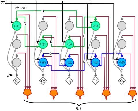
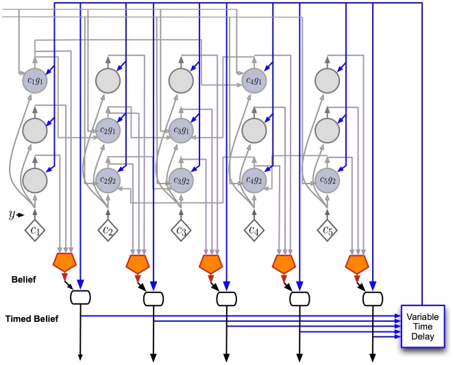
- The authors derive belief-propagation equations for an HTM node using coincidence patterns and Markov chains, then propose a cortical mapping: layer 4 stellate cells for coincidence likelihood, layer 2/3 pyramidal cells for sequence states and feed-forward/feedback computations, layer 5 cells for belief and timing, and layer 6 cells for feedback messages to child regions.
- On the Pictures line-drawing dataset, an HTM with Markov-chain temporal pooling only at level 1 achieved 49% recognition accuracy; adding temporal pooling at higher levels increased accuracy to 72%, compared with 35% for a nearest-neighbor classifier using the same top-level training paradigm.
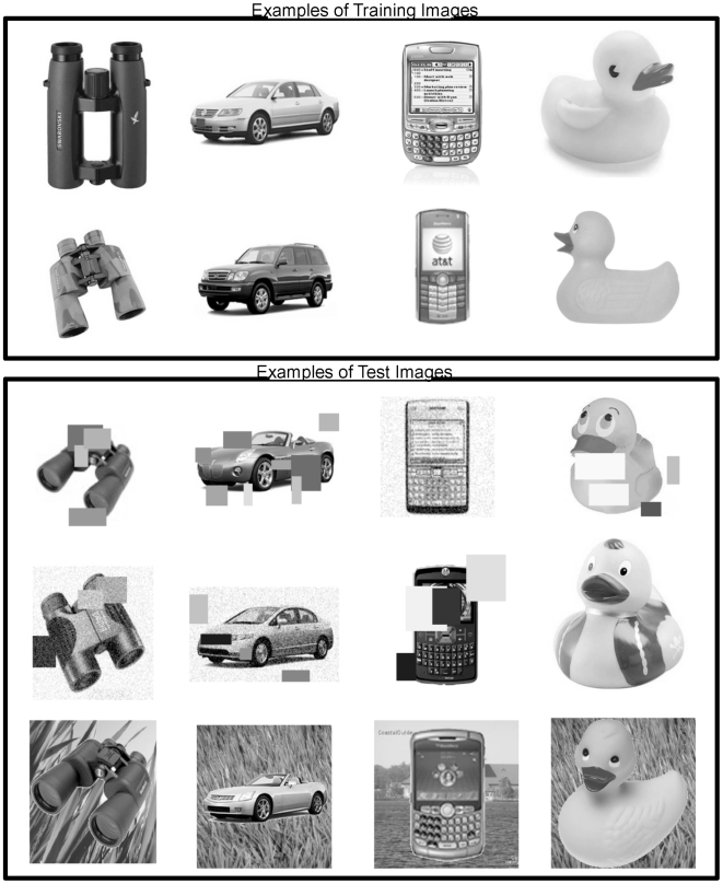
- On Caltech-101, initial HTM experiments achieved 50% recognition with 15 training images and 62% with 30 training images; on a 4-category grayscale set with over 10,000 training images, the network gave 92% accuracy on a holdout set. Temporal inference improved frame-by-frame recognition by up to 30% over sliding-window averaging (window length = 4).
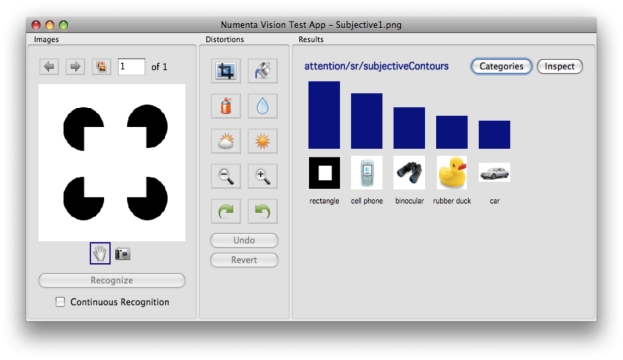
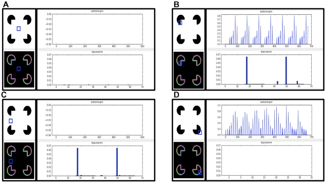
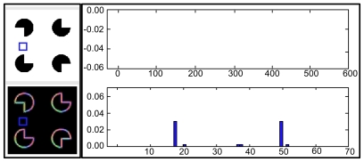
- In a Kanizsa square test, the network classified the pattern as a rectangle despite not being trained on Kanizsa squares; a node with no feed-forward contour input showed nonzero feedback, modeling the subjective contour effect, and a corrupted Kanizsa figure produced a weaker response.
Methods
- Theoretical/modeling study: starts from the HTM generative model, derives Bayesian belief-propagation equations for an HTM node, builds an abstract neuron-like circuit, and maps it onto cortical layers and columns by matching computational specifications with anatomical data.
- Experiments used Numenta’s NuPIC HTM networks for visual object recognition on the Pictures dataset (48 categories of 32×32 line drawings), Caltech-101, a 4-category grayscale dataset, temporal inference on Pictures, top-down segmentation, and subjective contour/Kanizsa tests.
- Analysis consisted of benchmark recognition-accuracy comparisons and qualitative inspection of node feed-forward and feedback states; no biological experiments are reported.
Limitations
- The paper states the model is a starting point, the biological mapping is not unique, and it does not address learning, attention, motor action, asynchronous messages, detailed dendritic properties, inhibitory cells, cortical maps, or sparse distributed representations within a node; it also assumes singly connected non-loopy networks for simplicity.
- The paper states the timing/duration mechanism is conjectural, the non-specific thalamic timing loop lacks direct evidence, no recordings from non-specific thalamic cells were found, and the subjective contour results are preliminary.
- Evident from the text: the biological predictions are largely untested, the benchmark experiments are from Numenta/NuPIC and not independent, and no statistical tests or error bars are reported for the recognition results.
Model-written summary. Check it against the paper before relying on it.
Integrity signals
Registry
Cites
Statistics
Figures
Verification
Claims the paper makes
163 Own interpretation · 79 Not checked yet · 21 Own result · 21 No basis given
In the paper
“We have found that a simple way to learn the mixture of Markov chains for real world cases is to learn a large transition matrix that is then partitioned using a graph partitioning algorithm [27].”
§ Towards a Mathematical Theory of Cortical Micro-circuits > Model > Hierarchical Temporal Memory
What the sources say
- Not checked yetcites [27] D George, 2007, The HTM Learning Algorithms
plaindirect- Asserted: passes — The authors put it forward as true.
- Checkable: passes — It can be checked against evidence.
- Load-bearing: unclear — It is unclear whether the paper’s conclusions depend on it.
- Based: passes — The paper gives a reason why it holds.
A result the paper reports from its own data — it cites no other source for it, so there is none to check. The quote shows it is in the paper.
In the paper
“we have found that storing a fixed number of a random selection of the coincidence patterns is sufficient as long as we allow multiple coincidence patterns to be active at the same time.”
§ Towards a Mathematical Theory of Cortical Micro-circuits > Model > Hierarchical Temporal Memory
plainconditional- Asserted: passes — The authors put it forward as true.
- Checkable: passes — It can be checked against evidence.
- Load-bearing: passes — The paper’s conclusions depend on it.
- Based: passes — The paper gives a reason why it holds.
A result the paper reports from its own data — it cites no other source for it, so there is none to check. The quote shows it is in the paper.
In the paper
“We have found that reasonable results can be achieved with a wide range of the number of coincidences stored.”
§ Towards a Mathematical Theory of Cortical Micro-circuits > Model > Hierarchical Temporal Memory
plain- Asserted: passes — The authors put it forward as true.
- Checkable: passes — It can be checked against evidence.
- Load-bearing: unclear — It is unclear whether the paper’s conclusions depend on it.
- Based: passes — The paper gives a reason why it holds.
A result the paper reports from its own data — it cites no other source for it, so there is none to check. The quote shows it is in the paper.
In the paper
“Our literature search and private conversations with several thalamic anatomists have yielded no evidence of anyone ever recording from non-specific thalamic cells.”
§ Towards a Mathematical Theory of Cortical Micro-circuits > Results > A detailed proposal for the computations performed by cortical layers
plain- Asserted: passes — The authors put it forward as true.
- Checkable: passes — It can be checked against evidence.
- Load-bearing: passes — The paper’s conclusions depend on it.
- Based: unclear — It is unclear why the paper says it holds.
The paper states this without a source or data behind it here, so there is nothing to check it against. The quote shows it is in the paper.
In the paper
“When we looked for anatomical data that satisfied these constraints, the cortical projections to and from non-specific thalamic cells were the best fit.”
§ Towards a Mathematical Theory of Cortical Micro-circuits > Results > A detailed proposal for the computations performed by cortical layers
plaincorrelational- Asserted: passes — The authors put it forward as true.
- Checkable: passes — It can be checked against evidence.
- Load-bearing: passes — The paper’s conclusions depend on it.
- Based: passes — The paper gives a reason why it holds.
The paper states this without a source or data behind it here, so there is nothing to check it against. The quote shows it is in the paper.
In the paper
“Beyond this connectivity there is nothing else to support this conjecture.”
§ Towards a Mathematical Theory of Cortical Micro-circuits > Results > A detailed proposal for the computations performed by cortical layers
plain- Asserted: passes — The authors put it forward as true.
- Checkable: passes — It can be checked against evidence.
- Load-bearing: unclear — It is unclear whether the paper’s conclusions depend on it.
- Based: passes — The paper gives a reason why it holds.
In the paper
“In this section, we report some preliminary positive results that we obtained modeling the subjective contour effect in visual inference [63] using these circuits.”
§ Towards a Mathematical Theory of Cortical Micro-circuits > Results > Example application: a model for the subjective contour effect
What the sources say
- Not checked yetcites [63] G Kanizsa, 1976, Subjective contours., Sci Am source
hedged- Asserted: passes — The authors put it forward as true.
- Checkable: passes — It can be checked against evidence.
- Load-bearing: unclear — It is unclear whether the paper’s conclusions depend on it.
- Based: passes — The paper gives a reason why it holds.
A result the paper reports from its own data — it cites no other source for it, so there is none to check. The quote shows it is in the paper.
In the paper
“Adding more levels did not help in improving the recognition accuracy on our test set.”
§ Towards a Mathematical Theory of Cortical Micro-circuits > Results > Object recognition experiments using HTMs
plain- Asserted: passes — The authors put it forward as true.
- Checkable: passes — It can be checked against evidence.
- Load-bearing: unclear — It is unclear whether the paper’s conclusions depend on it.
- Based: passes — The paper gives a reason why it holds.
A result the paper reports from its own data — it cites no other source for it, so there is none to check. The quote shows it is in the paper.
In the paper
“the corrupted rectangle produces a subjective contour response similar to, but substantially weaker than, the one produced by an intact Kanizsa figure.”
§ Towards a Mathematical Theory of Cortical Micro-circuits > Results > Example application: a model for the subjective contour effect
plaincorrelationalSingle case- Asserted: passes — The authors put it forward as true.
- Checkable: passes — It can be checked against evidence.
- Load-bearing: passes — The paper’s conclusions depend on it.
- Based: passes — The paper gives a reason why it holds.
A result the paper reports from its own data — it cites no other source for it, so there is none to check. The quote shows it is in the paper.
In the paper
“Only intact rectangle images were shown during training. The network then recognized novel rectangles of different aspect ratios.”
§ Towards a Mathematical Theory of Cortical Micro-circuits > Results > Example application: a model for the subjective contour effect
plaindirect- Asserted: passes — The authors put it forward as true.
- Checkable: passes — It can be checked against evidence.
- Load-bearing: unclear — It is unclear whether the paper’s conclusions depend on it.
- Based: passes — The paper gives a reason why it holds.
The paper states this without a source or data behind it here, so there is nothing to check it against. The quote shows it is in the paper.
In the paper
“Even with the combination of computational constraints and available anatomical data, several degrees of freedom remain in the mapping to biology.”
§ Towards a Mathematical Theory of Cortical Micro-circuits > Discussion
plain- Asserted: passes — The authors put it forward as true.
- Checkable: passes — It can be checked against evidence.
- Load-bearing: passes — The paper’s conclusions depend on it.
- Based: passes — The paper gives a reason why it holds.
A result the paper reports from its own data — it cites no other source for it, so there is none to check. The quote shows it is in the paper.
In the paper
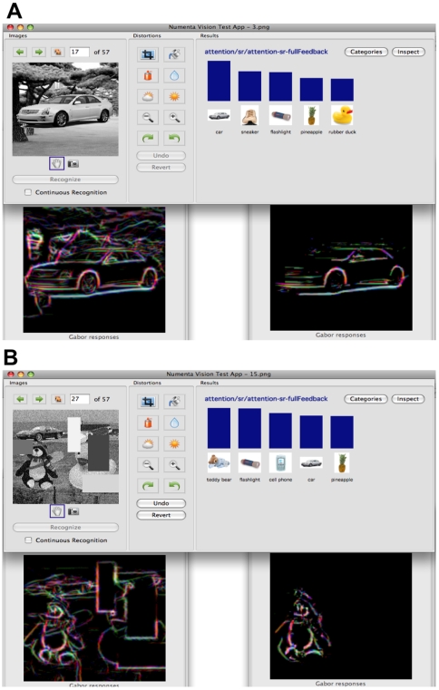
“In most cases, one of the objects in the test image was the top result in the inference.”
§ Towards a Mathematical Theory of Cortical Micro-circuits > Results > Object recognition experiments using HTMs
plain- Asserted: passes — The authors put it forward as true.
- Checkable: passes — It can be checked against evidence.
- Load-bearing: passes — The paper’s conclusions depend on it.
- Based: passes — The paper gives a reason why it holds.
The paper states this without a source or data behind it here, so there is nothing to check it against. The quote shows it is in the paper.
In the paper
“The circuits derived here attempt to explain only the information processing in a learned model.”
§ Towards a Mathematical Theory of Cortical Micro-circuits > Discussion
plain- Asserted: passes — The authors put it forward as true.
- Checkable: passes — It can be checked against evidence.
- Load-bearing: passes — The paper’s conclusions depend on it.
- Based: passes — The paper gives a reason why it holds.
A result the paper reports from its own data — it cites no other source for it, so there is none to check. The quote shows it is in the paper.
In the paper
“The resultant image obtained at the lowest level of the network isolates the contours of the recognized image from the background clutter and from other objects in the scene.”
§ Towards a Mathematical Theory of Cortical Micro-circuits > Results > Object recognition experiments using HTMs
plaindirect- Asserted: passes — The authors put it forward as true.
- Checkable: passes — It can be checked against evidence.
- Load-bearing: passes — The paper’s conclusions depend on it.
- Based: passes — The paper gives a reason why it holds.
The paper states this without a source or data behind it here, so there is nothing to check it against. The quote shows it is in the paper.
In the paper
“some of the intra-columnar vertical connections required to support the belief propagation equations can be pre-wired because these connections do not depend on external stimuli.”
§ Towards a Mathematical Theory of Cortical Micro-circuits > Discussion
plaindirect- Asserted: passes — The authors put it forward as true.
- Checkable: passes — It can be checked against evidence.
- Load-bearing: unclear — It is unclear whether the paper’s conclusions depend on it.
- Based: passes — The paper gives a reason why it holds.
A result the paper reports from its own data — it cites no other source for it, so there is none to check. The quote shows it is in the paper.
In the paper
“our limited experience with implementing overlapping input fields have similarly shown no tendency for loop-induced failures.”
§ Towards a Mathematical Theory of Cortical Micro-circuits > Discussion
hedged- Asserted: passes — The authors put it forward as true.
- Checkable: passes — It can be checked against evidence.
- Load-bearing: unclear — It is unclear whether the paper’s conclusions depend on it.
- Based: passes — The paper gives a reason why it holds.
A result the paper reports from its own data — it cites no other source for it, so there is none to check. The quote shows it is in the paper.
In the paper
“We found that HTM network hierarchies with four levels work best for the Pictures task.”
§ Towards a Mathematical Theory of Cortical Micro-circuits > Results > Object recognition experiments using HTMs
plaincorrelational- Asserted: passes — The authors put it forward as true.
- Checkable: passes — It can be checked against evidence.
- Load-bearing: unclear — It is unclear whether the paper’s conclusions depend on it.
- Based: passes — The paper gives a reason why it holds.
The paper states this without a source or data behind it here, so there is nothing to check it against. The quote shows it is in the paper.
In the paper
“Most other connections, the ones representing sequence memories and coincidence patterns, are learned.”
§ Towards a Mathematical Theory of Cortical Micro-circuits > Discussion
plain- Asserted: passes — The authors put it forward as true.
- Checkable: passes — It can be checked against evidence.
- Load-bearing: unclear — It is unclear whether the paper’s conclusions depend on it.
- Based: passes — The paper gives a reason why it holds.
A result the paper reports from its own data — it cites no other source for it, so there is none to check. The quote shows it is in the paper.
In the paper
“We found that incorporating Markov chains based temporal pooling at higher levels increased the recognition accuracy on test sets to 72%.”
§ Towards a Mathematical Theory of Cortical Micro-circuits > Results > Object recognition experiments using HTMs
plaindirect- Asserted: passes — The authors put it forward as true.
- Checkable: passes — It can be checked against evidence.
- Load-bearing: passes — The paper’s conclusions depend on it.
- Based: passes — The paper gives a reason why it holds.
A result the paper reports from its own data — it cites no other source for it, so there is none to check. The quote shows it is in the paper.
In the paper
“The recognition accuracy of the network that used temporal inference was up to 30% higher compared to the recognition accuracy obtained by a sliding window averaging (window length = 4) of frame-by-frame instantaneous recognition.”
§ Towards a Mathematical Theory of Cortical Micro-circuits > Results > Object recognition experiments using HTMs
plaindirect- Asserted: passes — The authors put it forward as true.
- Checkable: passes — It can be checked against evidence.
- Load-bearing: passes — The paper’s conclusions depend on it.
- Based: passes — The paper gives a reason why it holds.
A result the paper reports from its own data — it cites no other source for it, so there is none to check. The quote shows it is in the paper.
In the paper
“In comparison, a nearest neighbor classifier using exactly the training paradigm used to train the top level of the HTM gives only 35% accuracy.”
§ Towards a Mathematical Theory of Cortical Micro-circuits > Results > Object recognition experiments using HTMs
plain- Asserted: passes — The authors put it forward as true.
- Checkable: passes — It can be checked against evidence.
- Load-bearing: unclear — It is unclear whether the paper’s conclusions depend on it.
- Based: passes — The paper gives a reason why it holds.
The paper states this without a source or data behind it here, so there is nothing to check it against. The quote shows it is in the paper.
In the paper
“The subjective contour effect in our model was generated exclusively by feedback circuits.”
§ Towards a Mathematical Theory of Cortical Micro-circuits > Results > Example application: a model for the subjective contour effect
plaindirect- Asserted: passes — The authors put it forward as true.
- Checkable: passes — It can be checked against evidence.
- Load-bearing: passes — The paper’s conclusions depend on it.
- Based: passes — The paper gives a reason why it holds.
A result the paper reports from its own data — it cites no other source for it, so there is none to check. The quote shows it is in the paper.
In the paper
“With these modifications, we could successfully train several gray scale image recognition networks.”
§ Towards a Mathematical Theory of Cortical Micro-circuits > Results > Object recognition experiments using HTMs
hedgeddirect- Asserted: passes — The authors put it forward as true.
- Checkable: passes — It can be checked against evidence.
- Load-bearing: passes — The paper’s conclusions depend on it.
- Based: passes — The paper gives a reason why it holds.
A result the paper reports from its own data — it cites no other source for it, so there is none to check. The quote shows it is in the paper.
In the paper
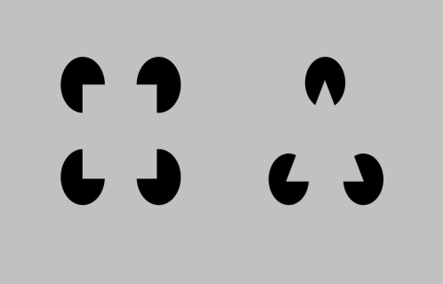
“There are no actual contours in the receptive field of this node. Therefore, the feed-forward input of this node is zero. However, the feedback input is nonzero because the network expects the edges of a rectangle. This is the subjective contour effect.”
§ Towards a Mathematical Theory of Cortical Micro-circuits > Results > Example application: a model for the subjective contour effect
plaindirectSingle case- Asserted: passes — The authors put it forward as true.
- Checkable: passes — It can be checked against evidence.
- Load-bearing: passes — The paper’s conclusions depend on it.
- Based: passes — The paper gives a reason why it holds.
A result the paper reports from its own data — it cites no other source for it, so there is none to check. The quote shows it is in the paper.
In the paper
“The network classifies this pattern as a rectangle, even though this type of pattern was not seen during training.”
§ Towards a Mathematical Theory of Cortical Micro-circuits > Results > Example application: a model for the subjective contour effect
plainSingle case- Asserted: passes — The authors put it forward as true.
- Checkable: passes — It can be checked against evidence.
- Load-bearing: passes — The paper’s conclusions depend on it.
- Based: passes — The paper gives a reason why it holds.
A result the paper reports from its own data — it cites no other source for it, so there is none to check. The quote shows it is in the paper.
In the paper
“In this paper we have mapped a model of how the neocortex performs inference onto neocortical anatomy.”
§ Towards a Mathematical Theory of Cortical Micro-circuits > Discussion > Conclusion
plaincorrelational- Asserted: passes — The authors put it forward as true.
- Checkable: passes — It can be checked against evidence.
- Load-bearing: passes — The paper’s conclusions depend on it.
- Based: passes — The paper gives a reason why it holds.
A result the paper reports from its own data — it cites no other source for it, so there is none to check. The quote shows it is in the paper.
In the paper
“We also showed results of an experiment where an HTM-based vision system exhibited the effects of illusory contours.”
§ Towards a Mathematical Theory of Cortical Micro-circuits > Discussion > Conclusion
plain- Asserted: passes — The authors put it forward as true.
- Checkable: passes — It can be checked against evidence.
- Load-bearing: unclear — It is unclear whether the paper’s conclusions depend on it.
- Based: passes — The paper gives a reason why it holds.
In the paper
“In addition, due to the temporal nature of HTM, this arrangement corresponds to a temporal hierarchy analogous to the kind reported by Hasson and colleagues [37].”
§ Towards a Mathematical Theory of Cortical Micro-circuits > Results > Mapping between neocortex hierarchy and HTM network hierarchy
What the sources say
- Not checked yetcites [37] U Hasson, 2008, A hierarchy of temporal receptive windows in human cortex., J Neurosci source
plaincorrelational- Asserted: passes — The authors put it forward as true.
- Checkable: passes — It can be checked against evidence.
- Load-bearing: unclear — It is unclear whether the paper’s conclusions depend on it.
- Based: passes — The paper gives a reason why it holds.
A conclusion the paper draws from its own results — it cites no other source for it, so there is none to check. The quote shows it is in the paper.
In the paper
“The feed-forward and feedback connections to a set of cortical columns carry the belief propagation messages.”
§ Towards a Mathematical Theory of Cortical Micro-circuits > Results > Mapping between neocortex hierarchy and HTM network hierarchy
plaindirect- Asserted: passes — The authors put it forward as true.
- Checkable: passes — It can be checked against evidence.
- Load-bearing: passes — The paper’s conclusions depend on it.
- Based: unclear — It is unclear why the paper says it holds.
- The authors state this as an assumption: The cortical circuits implement the HTM belief propagation equations described in Table 1.
A conclusion the paper draws from its own results — it cites no other source for it, so there is none to check. The quote shows it is in the paper.
In the paper
“The only difference between these two is the multiplication by a top-down factor in the belief calculation equations.”
§ Towards a Mathematical Theory of Cortical Micro-circuits > Model > Neuronal implementation of HTM belief propagation
plain- Asserted: passes — The authors put it forward as true.
- Checkable: passes — It can be checked against evidence.
- Load-bearing: passes — The paper’s conclusions depend on it.
- Based: passes — The paper gives a reason why it holds.
None of the sources cited for this claim have been checked yet.
In the paper
“However, they did not attempt to map these implementations to detailed cortical anatomy.”
§ Towards a Mathematical Theory of Cortical Micro-circuits > Introduction
What the sources say
- Not checked yetcites [4] S Deneve, 2005, Bayesian inference in spiking neurons, MIT Press.
- Not checked yetcites [13] RPN Rao, 2005, Hierarchical Bayesian Inference in Networks of Spiking Neurons, MIT Press.
plain- Asserted: passes — The authors put it forward as true.
- Checkable: passes — It can be checked against evidence.
- Load-bearing: passes — The paper’s conclusions depend on it.
- Based: passes — The paper gives a reason why it holds.
A conclusion the paper draws from its own results — it cites no other source for it, so there is none to check. The quote shows it is in the paper.
In the paper
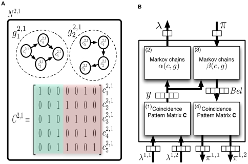
“Note that the operation of the rectangle neurons corresponds to pooling over the activations of all the circle neurons of the same Markov chain.”
§ Towards a Mathematical Theory of Cortical Micro-circuits > Model > Neuronal implementation of HTM belief propagation
plaindirect- Asserted: passes — The authors put it forward as true.
- Checkable: passes — It can be checked against evidence.
- Load-bearing: passes — The paper’s conclusions depend on it.
- Based: passes — The paper gives a reason why it holds.
A conclusion the paper draws from its own results — it cites no other source for it, so there is none to check. The quote shows it is in the paper.
In the paper
“Even though feedback propagation in the current model does not affect feed-forward propagation, it plays an important role in understanding the evidence presented to a network.”
§ Towards a Mathematical Theory of Cortical Micro-circuits > Model > Further considerations of belief propagation equations
plain- Asserted: passes — The authors put it forward as true.
- Checkable: passes — It can be checked against evidence.
- Load-bearing: unclear — It is unclear whether the paper’s conclusions depend on it.
- Based: passes — The paper gives a reason why it holds.
In the paper
“Belief propagation computations in poly tree structures have the property that the message from a child to a parent is influenced by the messages from all other parents to the child.”
§ Towards a Mathematical Theory of Cortical Micro-circuits > Model > Further considerations of belief propagation equations
What the sources say
- Not checked yetcites [29] J Pearl, 1988, Probabilistic Reasoning in Intelligent Systems: Networks of Plausible Inference
plaindirect- Asserted: passes — The authors put it forward as true.
- Checkable: passes — It can be checked against evidence.
- Load-bearing: passes — The paper’s conclusions depend on it.
- Based: passes — The paper gives a reason why it holds.
A conclusion the paper draws from its own results — it cites no other source for it, so there is none to check. The quote shows it is in the paper.
In the paper
“Therefore, higher-level cortical regions can possibly be modeled using a fewer number of HTM nodes.”
§ Towards a Mathematical Theory of Cortical Micro-circuits > Results > Mapping between neocortex hierarchy and HTM network hierarchy
hedgedconditional- Asserted: passes — The authors put it forward as true.
- Checkable: passes — It can be checked against evidence.
- Load-bearing: passes — The paper’s conclusions depend on it.
- Based: passes — The paper gives a reason why it holds.
- Rests on an assumption: The number of non-exclusive patterns that needs to be maintained decreases as you ascend in the hierarchy.
A conclusion the paper draws from its own results — it cites no other source for it, so there is none to check. The quote shows it is in the paper.
In the paper
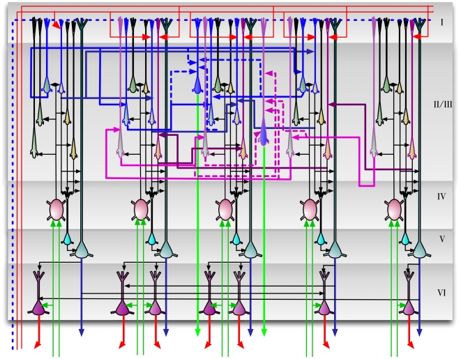
“The circuits in Figure 9 provide an exemplar instantiation of the Bayesian computations in laminar and columnar biological cortical circuits.”
§ Towards a Mathematical Theory of Cortical Micro-circuits > Results > A detailed proposal for the computations performed by cortical layers
plain- Asserted: passes — The authors put it forward as true.
- Checkable: passes — It can be checked against evidence.
- Load-bearing: passes — The paper’s conclusions depend on it.
- Based: unclear — It is unclear why the paper says it holds.
- The authors state this as an assumption: The cortical circuits implement the HTM belief propagation equations described in Table 1.
A conclusion the paper draws from its own results — it cites no other source for it, so there is none to check. The quote shows it is in the paper.
In the paper
“It is easy to verify that this is the operation involved in the calculation of the message this node sends to its parent according to Equation 3.”
§ Towards a Mathematical Theory of Cortical Micro-circuits > Model > Neuronal implementation of HTM belief propagation
plaindirect- Asserted: passes — The authors put it forward as true.
- Checkable: passes — It can be checked against evidence.
- Load-bearing: passes — The paper’s conclusions depend on it.
- Based: passes — The paper gives a reason why it holds.
In the paper
“HTM nodes with multiple parents can be treated like the causal poly-tree structures described by Pearl [29].”
§ Towards a Mathematical Theory of Cortical Micro-circuits > Model > Further considerations of belief propagation equations
What the sources say
- Not checked yetcites [29] J Pearl, 1988, Probabilistic Reasoning in Intelligent Systems: Networks of Plausible Inference
plaincorrelational- Asserted: passes — The authors put it forward as true.
- Checkable: passes — It can be checked against evidence.
- Load-bearing: unclear — It is unclear whether the paper’s conclusions depend on it.
- Based: passes — The paper gives a reason why it holds.
In the paper
“However, these models do not incorporate the concepts of Bayesian inference in a hierarchical temporal model.”
§ Towards a Mathematical Theory of Cortical Micro-circuits > Introduction
What the sources say
- Not checked yetcites [10]–[12]
plain- Asserted: passes — The authors put it forward as true.
- Checkable: passes — It can be checked against evidence.
- Load-bearing: passes — The paper’s conclusions depend on it.
- Based: passes — The paper gives a reason why it holds.
A conclusion the paper draws from its own results — it cites no other source for it, so there is none to check. The quote shows it is in the paper.
In the paper
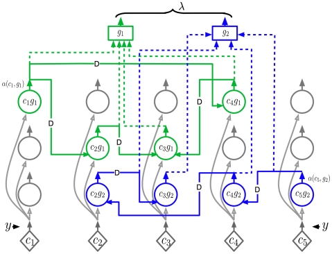
“Therefore, the neuronal implementation of the dynamic programming part of the belief calculation equation is very similar to that of the forward dynamic programming variable .”
§ Towards a Mathematical Theory of Cortical Micro-circuits > Model > Neuronal implementation of HTM belief propagation
plaincorrelational- Asserted: passes — The authors put it forward as true.
- Checkable: passes — It can be checked against evidence.
- Load-bearing: unclear — It is unclear whether the paper’s conclusions depend on it.
- Based: passes — The paper gives a reason why it holds.
A conclusion the paper draws from its own results — it cites no other source for it, so there is none to check. The quote shows it is in the paper.
In the paper
“The neurons in each column represent some aspect of the coincidence pattern that the column represents.”
§ Towards a Mathematical Theory of Cortical Micro-circuits > Results > A detailed proposal for the computations performed by cortical layers
plaincorrelational- Asserted: passes — The authors put it forward as true.
- Checkable: passes — It can be checked against evidence.
- Load-bearing: passes — The paper’s conclusions depend on it.
- Based: passes — The paper gives a reason why it holds.
- The authors state this as an assumption: The cortical circuits implement the HTM belief propagation equations described in Table 1.
A conclusion the paper draws from its own results — it cites no other source for it, so there is none to check. The quote shows it is in the paper.
In the paper
“To calculate efficiently, all the past evidence needs to be collapsed into a state variable that can be updated recursively every time instant.”
§ Towards a Mathematical Theory of Cortical Micro-circuits > Model > Neuronal implementation of HTM belief propagation
plaindirect- Asserted: passes — The authors put it forward as true.
- Checkable: passes — It can be checked against evidence.
- Load-bearing: passes — The paper’s conclusions depend on it.
- Based: passes — The paper gives a reason why it holds.
None of the sources cited for this claim have been checked yet.
In the paper
“Even though theoretical guarantees do not exist for belief propagation in loopy graphs, it is found to work well in practice on many problems involving loops [32],[33].”
§ Towards a Mathematical Theory of Cortical Micro-circuits > Model > Further considerations of belief propagation equations
What the sources say
- Not checked yetcites [32] BJ Frey, 1998, A revolution: Belief propagation in graphs with cycles.
- Not checked yetcites [33] K Murphy, 2000, Loopy-belief propagation for approximate inference: An empirical study.
plain- Asserted: passes — The authors put it forward as true.
- Checkable: passes — It can be checked against evidence.
- Load-bearing: unclear — It is unclear whether the paper’s conclusions depend on it.
- Based: passes — The paper gives a reason why it holds.
In the paper
“This arrangement corresponds to one of the basic organizing principles of the visual system where neurons in higher-level visual areas receive inputs from many neurons with smaller receptive fields in lower-level visual areas [36].”
§ Towards a Mathematical Theory of Cortical Micro-circuits > Results > Mapping between neocortex hierarchy and HTM network hierarchy
What the sources say
- Not checked yetcites [36] D Hubel, 1988, Eye, brain, and vision
plaincorrelational- Asserted: passes — The authors put it forward as true.
- Checkable: passes — It can be checked against evidence.
- Load-bearing: unclear — It is unclear whether the paper’s conclusions depend on it.
- Based: passes — The paper gives a reason why it holds.
A conclusion the paper draws from its own results — it cites no other source for it, so there is none to check. The quote shows it is in the paper.
In the paper
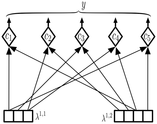
“Equation 4 can have a very efficient neuronal implementation as shown in Figure 4.”
§ Towards a Mathematical Theory of Cortical Micro-circuits > Model > Neuronal implementation of HTM belief propagation
plain- Asserted: passes — The authors put it forward as true.
- Checkable: passes — It can be checked against evidence.
- Load-bearing: unclear — It is unclear whether the paper’s conclusions depend on it.
- Based: passes — The paper gives a reason why it holds.
The paper states this without a source or data behind it here, so there is nothing to check it against. The quote shows it is in the paper.
In the paper
“To our knowledge, the work in this paper is the first attempt to map the theory of Bayesian belief propagation and hierarchical and temporal inference onto cortical circuitry.”
§ Towards a Mathematical Theory of Cortical Micro-circuits > Introduction
hedged- Asserted: passes — The authors put it forward as true.
- Checkable: passes — It can be checked against evidence.
- Load-bearing: passes — The paper’s conclusions depend on it.
- Based: passes — The paper gives a reason why it holds.
A conclusion the paper draws from its own results — it cites no other source for it, so there is none to check. The quote shows it is in the paper.
In the paper
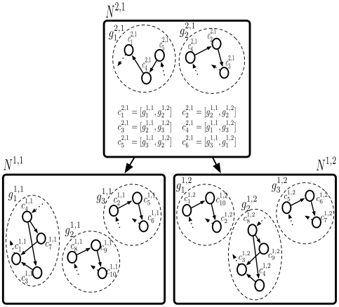
“A region of cortex that has several patterns simultaneously active will be implemented using several HTM nodes.”
§ Towards a Mathematical Theory of Cortical Micro-circuits > Results > Mapping between neocortex hierarchy and HTM network hierarchy
plaindirect- Asserted: passes — The authors put it forward as true.
- Checkable: passes — It can be checked against evidence.
- Load-bearing: passes — The paper’s conclusions depend on it.
- Based: passes — The paper gives a reason why it holds.
- The authors state this as an assumption: The cortical circuits implement the HTM belief propagation equations described in Table 1.
A conclusion the paper draws from its own results — it cites no other source for it, so there is none to check. The quote shows it is in the paper.
In the paper
“In this paper, we describe how Bayesian belief propagation in a spatio-temporal hierarchical model, called Hierarchical Temporal Memory (HTM), can lead to a mathematical model for cortical circuits.”
§ Towards a Mathematical Theory of Cortical Micro-circuits > Abstract
plaindirect- Asserted: passes — The authors put it forward as true.
- Checkable: passes — It can be checked against evidence.
- Load-bearing: passes — The paper’s conclusions depend on it.
- Based: passes — The paper gives a reason why it holds.
A conclusion the paper draws from its own results — it cites no other source for it, so there is none to check. The quote shows it is in the paper.
In the paper
“If the receptive field is small enough, the different orientations can be considered mutually exclusive - the activity of one reduces the activity of the other.”
§ Towards a Mathematical Theory of Cortical Micro-circuits > Results > A detailed proposal for the computations performed by cortical layers
plaindirect- Asserted: passes — The authors put it forward as true.
- Checkable: passes — It can be checked against evidence.
- Load-bearing: passes — The paper’s conclusions depend on it.
- Based: unclear — It is unclear why the paper says it holds.
In the paper
“Multiple top-down causes can be combined efficiently using the noisy OR-gate structures described in Pearl's book [29].”
§ Towards a Mathematical Theory of Cortical Micro-circuits > Model > Further considerations of belief propagation equations
What the sources say
- Not checked yetcites [29] J Pearl, 1988, Probabilistic Reasoning in Intelligent Systems: Networks of Plausible Inference
plaindirect- Asserted: passes — The authors put it forward as true.
- Checkable: passes — It can be checked against evidence.
- Load-bearing: unclear — It is unclear whether the paper’s conclusions depend on it.
- Based: passes — The paper gives a reason why it holds.
A conclusion the paper draws from its own results — it cites no other source for it, so there is none to check. The quote shows it is in the paper.
In the paper
“A brute-force computation of this quantity is not feasible because this requires the enumeration of the likelihoods of an exponentially growing number of sample paths.”
§ Towards a Mathematical Theory of Cortical Micro-circuits > Model > Neuronal implementation of HTM belief propagation
plaindirect- Asserted: passes — The authors put it forward as true.
- Checkable: passes — It can be checked against evidence.
- Load-bearing: passes — The paper’s conclusions depend on it.
- Based: passes — The paper gives a reason why it holds.
In the paper
“However, there still remains a gap between our understanding of learning and inference in hierarchical Bayesian models and our understanding of how it is implemented in cortical circuits.”
§ Towards a Mathematical Theory of Cortical Micro-circuits > Introduction
What the sources say
- Not checked yetcites [2] J Hegde, 2007, Reappraising the functional implications of the primate visual anatomical hierarchy., Neuroscientist source
plain- Asserted: passes — The authors put it forward as true.
- Checkable: passes — It can be checked against evidence.
- Load-bearing: passes — The paper’s conclusions depend on it.
- Based: passes — The paper gives a reason why it holds.
A conclusion the paper draws from its own results — it cites no other source for it, so there is none to check. The quote shows it is in the paper.
In the paper
“Bayesian belief propagation equations for such an HTM node define a set of functional constraints for a neuronal implementation.”
§ Towards a Mathematical Theory of Cortical Micro-circuits > Abstract
plaindirect- Asserted: passes — The authors put it forward as true.
- Checkable: passes — It can be checked against evidence.
- Load-bearing: passes — The paper’s conclusions depend on it.
- Based: passes — The paper gives a reason why it holds.
A conclusion the paper draws from its own results — it cites no other source for it, so there is none to check. The quote shows it is in the paper.
In the paper
“Since an HTM node abstracts space as well as time, new equations must be derived for belief propagation in HTM nodes.”
§ Towards a Mathematical Theory of Cortical Micro-circuits > Model > Hierarchical Temporal Memory
plaindirect- Asserted: passes — The authors put it forward as true.
- Checkable: passes — It can be checked against evidence.
- Load-bearing: passes — The paper’s conclusions depend on it.
- Based: passes — The paper gives a reason why it holds.
A conclusion the paper draws from its own results — it cites no other source for it, so there is none to check. The quote shows it is in the paper.
In the paper
“Even though feedback propagation in the current model does not affect feed-forward propagation, it plays an important role in understanding the evidence presented to a network.”
§ Towards a Mathematical Theory of Cortical Micro-circuits > Model > Further considerations of belief propagation equations
plain- Asserted: passes — The authors put it forward as true.
- Checkable: passes — It can be checked against evidence.
- Load-bearing: unclear — It is unclear whether the paper’s conclusions depend on it.
- Based: passes — The paper gives a reason why it holds.
In the paper
“However, self-loops lead to an exponential duration probability density that is inappropriate for most physical signals [35].”
§ Towards a Mathematical Theory of Cortical Micro-circuits > Model > Further considerations of belief propagation equations
What the sources say
- Not checked yetcites [35] LR Rabiner, 1989, A tutorial on hidden Markov models and selected applications in speech recognition., Proceedings of the IEEE source
plaindirect- Asserted: passes — The authors put it forward as true.
- Checkable: passes — It can be checked against evidence.
- Load-bearing: passes — The paper’s conclusions depend on it.
- Based: passes — The paper gives a reason why it holds.
A conclusion the paper draws from its own results — it cites no other source for it, so there is none to check. The quote shows it is in the paper.
In the paper
“It is easy to verify that the connections of these neurons correspond to the ‘diamond’ neurons in our belief propagation implementation shown in Figures 3 , 4 and 5.”
§ Towards a Mathematical Theory of Cortical Micro-circuits > Results > A detailed proposal for the computations performed by cortical layers
boostedcorrelational- Asserted: passes — The authors put it forward as true.
- Checkable: passes — It can be checked against evidence.
- Load-bearing: passes — The paper’s conclusions depend on it.
- Based: passes — The paper gives a reason why it holds.
- The authors state this as an assumption: The cortical circuits implement the HTM belief propagation equations described in Table 1.
In the paper
“The major excitatory projection of layer 4 neurons is to layer 2/3 neurons [45].”
§ Towards a Mathematical Theory of Cortical Micro-circuits > Results > A detailed proposal for the computations performed by cortical layers
What the sources say
- Not checked yetcites [45] AM Thomson, 2007, Functional maps of neocortical local circuitry., Front Neurosci source
plaindirect- Asserted: passes — The authors put it forward as true.
- Checkable: passes — It can be checked against evidence.
- Load-bearing: passes — The paper’s conclusions depend on it.
- Based: passes — The paper gives a reason why it holds.
None of the sources cited for this claim have been checked yet.
In the paper
“Feedback connections from higher levels of the cortex rise to layer 1.”
§ Towards a Mathematical Theory of Cortical Micro-circuits > Results > A detailed proposal for the computations performed by cortical layers
plaindirect- Asserted: passes — The authors put it forward as true.
- Checkable: passes — It can be checked against evidence.
- Load-bearing: passes — The paper’s conclusions depend on it.
- Based: passes — The paper gives a reason why it holds.
A conclusion the paper draws from its own results — it cites no other source for it, so there is none to check. The quote shows it is in the paper.
In the paper
“A coincidence that is represented by a single neuron in our cortical column can be represented by a cluster of laterally interconnected neurons.”
§ Towards a Mathematical Theory of Cortical Micro-circuits > Results > A detailed proposal for the computations performed by cortical layers
plaincorrelational- Asserted: passes — The authors put it forward as true.
- Checkable: passes — It can be checked against evidence.
- Load-bearing: passes — The paper’s conclusions depend on it.
- Based: passes — The paper gives a reason why it holds.
A conclusion the paper draws from its own results — it cites no other source for it, so there is none to check. The quote shows it is in the paper.
In the paper
“We propose three different roles for the layer 2/3 pyramidal neurons in cortical circuits: (1) Calculation of feed-forward Markov chain (sequence) states, (2) Projection of Markov chain information to higher level cortical areas, and (3) Computation of sequence states that incorporate feedback information.”
§ Towards a Mathematical Theory of Cortical Micro-circuits > Results > A detailed proposal for the computations performed by cortical layers
plaindirect- Asserted: passes — The authors put it forward as true.
- Checkable: passes — It can be checked against evidence.
- Load-bearing: passes — The paper’s conclusions depend on it.
- Based: unclear — It is unclear why the paper says it holds.
- The authors state this as an assumption: The cortical circuits implement the HTM belief propagation equations described in Table 1.
A conclusion the paper draws from its own results — it cites no other source for it, so there is none to check. The quote shows it is in the paper.
In the paper
“This means that layer 4 neurons are coincidence detectors and that the synapses of the layer 4 neurons represent co-occurrence patterns on its inputs.”
§ Towards a Mathematical Theory of Cortical Micro-circuits > Results > A detailed proposal for the computations performed by cortical layers
plaincorrelational- Asserted: passes — The authors put it forward as true.
- Checkable: passes — It can be checked against evidence.
- Load-bearing: passes — The paper’s conclusions depend on it.
- Based: passes — The paper gives a reason why it holds.
- The authors state this as an assumption: The cortical circuits implement the HTM belief propagation equations described in Table 1.
A conclusion the paper draws from its own results — it cites no other source for it, so there is none to check. The quote shows it is in the paper.
In the paper
“We propose a third set of pyramidal neurons in layer 2/3 for this purpose.”
§ Towards a Mathematical Theory of Cortical Micro-circuits > Results > A detailed proposal for the computations performed by cortical layers
plaindirect- Asserted: passes — The authors put it forward as true.
- Checkable: passes — It can be checked against evidence.
- Load-bearing: passes — The paper’s conclusions depend on it.
- Based: passes — The paper gives a reason why it holds.
- The authors state this as an assumption: The cortical circuits implement the HTM belief propagation equations described in Table 1.
A conclusion the paper draws from its own results — it cites no other source for it, so there is none to check. The quote shows it is in the paper.
In the paper
“These connections act as a backbone for carrying out belief propagation computations.”
§ Towards a Mathematical Theory of Cortical Micro-circuits > Results > A detailed proposal for the computations performed by cortical layers
plaindirect- Asserted: passes — The authors put it forward as true.
- Checkable: passes — It can be checked against evidence.
- Load-bearing: passes — The paper’s conclusions depend on it.
- Based: passes — The paper gives a reason why it holds.
- The authors state this as an assumption: The cortical circuits implement the HTM belief propagation equations described in Table 1.
None of the sources cited for this claim have been checked yet.
In the paper
“We found several data points suggesting that neurons in layer 2/3 are capable of approximating a similar computation.”
§ Towards a Mathematical Theory of Cortical Micro-circuits > Results > A detailed proposal for the computations performed by cortical layers
What the sources say
- Not checked yetcites [49] Y Yoshimura, 2000, Properties of horizontal and vertical inputs to pyramidal cells in the superficial layers of the cat visual cortex., Journal of Neuroscience source
- Not checked yetcites [50] D Feldmeyer, 2002, Synaptic connections between layer 4 spiny neurone-layer 2/3 pyramidal cell pairs in juvenile rat barrel cortex: physiology and anatomy of interlaminar signalling within a cortical column., The Journal of Physiology source
hedgedcorrelational- Asserted: passes — The authors put it forward as true.
- Checkable: passes — It can be checked against evidence.
- Load-bearing: passes — The paper’s conclusions depend on it.
- Based: passes — The paper gives a reason why it holds.
In the paper
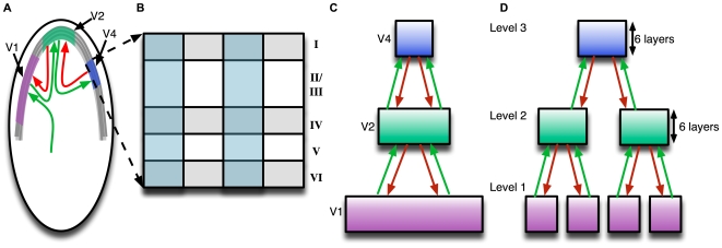
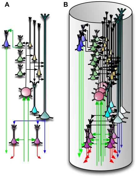
“The idealized cortical column in Figure 10(A) can correspond to what is known as the mini-columns or ontogenetic columns of the cortex [40].”
§ Towards a Mathematical Theory of Cortical Micro-circuits > Results > A detailed proposal for the computations performed by cortical layers
What the sources say
- Not checked yetcites [40] P Rakic, 1988, Specification of cerebral cortical areas., Science source
plaincorrelational- Asserted: passes — The authors put it forward as true.
- Checkable: passes — It can be checked against evidence.
- Load-bearing: unclear — It is unclear whether the paper’s conclusions depend on it.
- Based: passes — The paper gives a reason why it holds.
In the paper
“For example, L4 spiny neurons in the barrel cortex of the mouse are characterized by mainly vertically-oriented, predominantly intra-columnar, axons that target layer 2/3 pyramidal cells [46].”
§ Towards a Mathematical Theory of Cortical Micro-circuits > Results > A detailed proposal for the computations performed by cortical layers
What the sources say
- Not checked yetcites [46] J Lubke, 2007, Excitatory signal flow and connectivity in a cortical column: focus on barrel cortex., Brain Struct Funct source
plaincorrelational- Asserted: passes — The authors put it forward as true.
- Checkable: passes — It can be checked against evidence.
- Load-bearing: passes — The paper’s conclusions depend on it.
- Based: passes — The paper gives a reason why it holds.
A conclusion the paper draws from its own results — it cites no other source for it, so there is none to check. The quote shows it is in the paper.
In the paper
“They become most active only in the context of the correct sequence.”
§ Towards a Mathematical Theory of Cortical Micro-circuits > Results > A detailed proposal for the computations performed by cortical layers
plaincorrelational- Asserted: passes — The authors put it forward as true.
- Checkable: passes — It can be checked against evidence.
- Load-bearing: passes — The paper’s conclusions depend on it.
- Based: passes — The paper gives a reason why it holds.
- The authors state this as an assumption: The cortical circuits implement the HTM belief propagation equations described in Table 1.
A conclusion the paper draws from its own results — it cites no other source for it, so there is none to check. The quote shows it is in the paper.
In the paper
“The axons carrying feedback information will be available at layer 1 and accessed by the apical dendrites of neurons that require this information.”
§ Towards a Mathematical Theory of Cortical Micro-circuits > Results > A detailed proposal for the computations performed by cortical layers
plaindirect- Asserted: passes — The authors put it forward as true.
- Checkable: passes — It can be checked against evidence.
- Load-bearing: passes — The paper’s conclusions depend on it.
- Based: passes — The paper gives a reason why it holds.
- The authors state this as an assumption: The cortical circuits implement the HTM belief propagation equations described in Table 1.
None of the sources cited for this claim have been checked yet.
In the paper
“In biology, it is found that axons of the layer 2/3 pyramidal neurons travel several millimeters parallel to the layer 2/3 – layer 4 boundary and re-enter layer 2/3 to make excitatory connections to pyramidal cells there [43],[48].”
§ Towards a Mathematical Theory of Cortical Micro-circuits > Results > A detailed proposal for the computations performed by cortical layers
What the sources say
- Not checked yetcites [43] PA Bannister, 2005, Inter- and intra-laminar connections of pyramidal cells in the neocortex., Neurosci Res source
- Not checked yetcites [48] JS Lund, 2003, Anatomical substrates for functional columns in macaque monkey primary visual cortex., Cerebral cortex (New York, NY : 1991)
plaindirect- Asserted: passes — The authors put it forward as true.
- Checkable: passes — It can be checked against evidence.
- Load-bearing: passes — The paper’s conclusions depend on it.
- Based: passes — The paper gives a reason why it holds.
In the paper
“They also found that when both the vertical and horizontal inputs were driven simultaneously, the evoked EPSP was larger than the mathematical summation of the individual EPSPs.”
§ Towards a Mathematical Theory of Cortical Micro-circuits > Results > A detailed proposal for the computations performed by cortical layers
What the sources say
- Not checked yetcites [49] Y Yoshimura, 2000, Properties of horizontal and vertical inputs to pyramidal cells in the superficial layers of the cat visual cortex., Journal of Neuroscience source
plaindirect- Asserted: passes — The authors put it forward as true.
- Checkable: passes — It can be checked against evidence.
- Load-bearing: passes — The paper’s conclusions depend on it.
- Based: passes — The paper gives a reason why it holds.
In the paper
“Unlike cells in layer 4 that respond to more impoverished stimuli, cells in layer 2/3 of the visual and barrel cortices strongly prefer richer stimuli, such as motion in the preferred direction [47].”
§ Towards a Mathematical Theory of Cortical Micro-circuits > Results > A detailed proposal for the computations performed by cortical layers
What the sources say
- Not checked yetcites [47] JA Hirsch, 2006, Laminar processing in the visual cortical column., Curr Opin Neurobiol source
boostedcorrelational- Asserted: passes — The authors put it forward as true.
- Checkable: passes — It can be checked against evidence.
- Load-bearing: passes — The paper’s conclusions depend on it.
- Based: passes — The paper gives a reason why it holds.
A conclusion the paper draws from its own results — it cites no other source for it, so there is none to check. The quote shows it is in the paper.
In the paper
“We propose three different roles for the layer 2/3 pyramidal neurons in cortical circuits: (1) Calculation of feed-forward Markov chain (sequence) states, (2) Projection of Markov chain information to higher level cortical areas, and (3) Computation of sequence states that incorporate feedback information.”
§ Towards a Mathematical Theory of Cortical Micro-circuits > Results > A detailed proposal for the computations performed by cortical layers
plaindirect- Asserted: passes — The authors put it forward as true.
- Checkable: passes — It can be checked against evidence.
- Load-bearing: passes — The paper’s conclusions depend on it.
- Based: unclear — It is unclear why the paper says it holds.
- The authors state this as an assumption: The cortical circuits implement the HTM belief propagation equations described in Table 1.
In the paper
“In neuroscience, it is accepted that the feedback inputs to a cortical region generally avoid layer 4 [2].”
§ Towards a Mathematical Theory of Cortical Micro-circuits > Results > A detailed proposal for the computations performed by cortical layers
What the sources say
- Not checked yetcites [2] J Hegde, 2007, Reappraising the functional implications of the primate visual anatomical hierarchy., Neuroscientist source
boosted- Asserted: passes — The authors put it forward as true.
- Checkable: passes — It can be checked against evidence.
- Load-bearing: passes — The paper’s conclusions depend on it.
- Based: passes — The paper gives a reason why it holds.
In the paper
“In addition, the layer 2/3 neurons receive excitatory inputs from other layer 2/3 neurons via extensive lateral connections [43].”
§ Towards a Mathematical Theory of Cortical Micro-circuits > Results > A detailed proposal for the computations performed by cortical layers
What the sources say
- Not checked yetcites [43] PA Bannister, 2005, Inter- and intra-laminar connections of pyramidal cells in the neocortex., Neurosci Res source
plaindirect- Asserted: passes — The authors put it forward as true.
- Checkable: passes — It can be checked against evidence.
- Load-bearing: passes — The paper’s conclusions depend on it.
- Based: passes — The paper gives a reason why it holds.
A conclusion the paper draws from its own results — it cites no other source for it, so there is none to check. The quote shows it is in the paper.
In the paper
“One prediction of our model is that many of the connections within a vertical column of cells can be established without any learning.”
§ Towards a Mathematical Theory of Cortical Micro-circuits > Results > A detailed proposal for the computations performed by cortical layers
plain- Asserted: passes — The authors put it forward as true.
- Checkable: passes — It can be checked against evidence.
- Load-bearing: passes — The paper’s conclusions depend on it.
- Based: passes — The paper gives a reason why it holds.
- The authors state this as an assumption: The cortical circuits implement the HTM belief propagation equations described in Table 1.
A conclusion the paper draws from its own results — it cites no other source for it, so there is none to check. The quote shows it is in the paper.
In the paper
“This means that there is no redundancy in this idealized cortical representation.”
§ Towards a Mathematical Theory of Cortical Micro-circuits > Results > A detailed proposal for the computations performed by cortical layers
plain- Asserted: passes — The authors put it forward as true.
- Checkable: passes — It can be checked against evidence.
- Load-bearing: unclear — It is unclear whether the paper’s conclusions depend on it.
- Based: passes — The paper gives a reason why it holds.
A conclusion the paper draws from its own results — it cites no other source for it, so there is none to check. The quote shows it is in the paper.
In the paper
“A prediction arising from this mechanism is that two classes of neurons in layer 2/3 can be differentiated by the connections they make in layer 1.”
§ Towards a Mathematical Theory of Cortical Micro-circuits > Results > A detailed proposal for the computations performed by cortical layers
plaincorrelational- Asserted: passes — The authors put it forward as true.
- Checkable: passes — It can be checked against evidence.
- Load-bearing: passes — The paper’s conclusions depend on it.
- Based: passes — The paper gives a reason why it holds.
- The authors state this as an assumption: The cortical circuits implement the HTM belief propagation equations described in Table 1.
In the paper
“The excitatory neurons in layer 4 of the cortex consist primarily of star-shaped neurons called stellate neurons and pyramidal neurons [42].”
§ Towards a Mathematical Theory of Cortical Micro-circuits > Results > A detailed proposal for the computations performed by cortical layers
What the sources say
- Not checked yetcites [42] AM Thomson, 2003, Interlaminar connections in the neocortex., Cerebral cortex (New York, NY : 1991)
plain- Asserted: passes — The authors put it forward as true.
- Checkable: passes — It can be checked against evidence.
- Load-bearing: unclear — It is unclear whether the paper’s conclusions depend on it.
- Based: passes — The paper gives a reason why it holds.
In the paper
“Many layer 2/3 neurons project to higher levels of cortex and to layer 5 [44].”
§ Towards a Mathematical Theory of Cortical Micro-circuits > Results > A detailed proposal for the computations performed by cortical layers
What the sources say
- Not checked yetcites [44] AM Thomson, 1998, Postsynaptic pyramidal target selection by descending layer iii pyramidal axons: dual intracellular recordings and biocytin filling in slices of rat neocortex., Neuroscience source
plain- Asserted: passes — The authors put it forward as true.
- Checkable: passes — It can be checked against evidence.
- Load-bearing: passes — The paper’s conclusions depend on it.
- Based: passes — The paper gives a reason why it holds.
In the paper
“By the 26th gestational week, the human neocortex is composed of a large number of mini-columns in parallel vertical arrays [41].”
§ Towards a Mathematical Theory of Cortical Micro-circuits > Results > A detailed proposal for the computations performed by cortical layers
What the sources say
- Not checked yetcites [41] VB Mountcastle, 2003, Introduction to the special issue on computation in cortical columns., Cerebral Cortex
plain- Asserted: passes — The authors put it forward as true.
- Checkable: passes — It can be checked against evidence.
- Load-bearing: passes — The paper’s conclusions depend on it.
- Based: passes — The paper gives a reason why it holds.
A conclusion the paper draws from its own results — it cites no other source for it, so there is none to check. The quote shows it is in the paper.
In the paper
“One class of layer 2/3 neuron will form layer 1 synapses with feedback axons from higher levels of cortex.”
§ Towards a Mathematical Theory of Cortical Micro-circuits > Results > A detailed proposal for the computations performed by cortical layers
plaincorrelational- Asserted: passes — The authors put it forward as true.
- Checkable: passes — It can be checked against evidence.
- Load-bearing: passes — The paper’s conclusions depend on it.
- Based: passes — The paper gives a reason why it holds.
- The authors state this as an assumption: The cortical circuits implement the HTM belief propagation equations described in Table 1.
A conclusion the paper draws from its own results — it cites no other source for it, so there is none to check. The quote shows it is in the paper.
In the paper
“However, these yellow layer 2/3 neurons also integrate feedback information from layer 1 using their apical dendrites in layer 1 as shown in Figure 9.”
§ Towards a Mathematical Theory of Cortical Micro-circuits > Results > A detailed proposal for the computations performed by cortical layers
plaindirect- Asserted: passes — The authors put it forward as true.
- Checkable: passes — It can be checked against evidence.
- Load-bearing: passes — The paper’s conclusions depend on it.
- Based: passes — The paper gives a reason why it holds.
- The authors state this as an assumption: The cortical circuits implement the HTM belief propagation equations described in Table 1.
In the paper
“They found that, under depolarized conditions, the EPSP evoked by the activation of an individual input pathway (either horizontal or vertical, but not both) was smaller than that evoked without the depolarization.”
§ Towards a Mathematical Theory of Cortical Micro-circuits > Results > A detailed proposal for the computations performed by cortical layers
What the sources say
- Not checked yetcites [49] Y Yoshimura, 2000, Properties of horizontal and vertical inputs to pyramidal cells in the superficial layers of the cat visual cortex., Journal of Neuroscience source
plaindirect- Asserted: passes — The authors put it forward as true.
- Checkable: passes — It can be checked against evidence.
- Load-bearing: passes — The paper’s conclusions depend on it.
- Based: passes — The paper gives a reason why it holds.
A conclusion the paper draws from its own results — it cites no other source for it, so there is none to check. The quote shows it is in the paper.
In the paper
“The computation that the sequence state cells in layer 2/3 need to perform for inference involves a weighted sum of their lateral connections multiplied by a bottom-up input.”
§ Towards a Mathematical Theory of Cortical Micro-circuits > Results > A detailed proposal for the computations performed by cortical layers
plaindirect- Asserted: passes — The authors put it forward as true.
- Checkable: passes — It can be checked against evidence.
- Load-bearing: passes — The paper’s conclusions depend on it.
- Based: passes — The paper gives a reason why it holds.
A conclusion the paper draws from its own results — it cites no other source for it, so there is none to check. The quote shows it is in the paper.
In the paper
“The axons from these pyramidal cells cross column boundaries and connect to other pyramidal neurons that belong to the same sequence.”
§ Towards a Mathematical Theory of Cortical Micro-circuits > Results > A detailed proposal for the computations performed by cortical layers
plaincorrelational- Asserted: passes — The authors put it forward as true.
- Checkable: passes — It can be checked against evidence.
- Load-bearing: passes — The paper’s conclusions depend on it.
- Based: unclear — It is unclear why the paper says it holds.
- The authors state this as an assumption: The cortical circuits implement the HTM belief propagation equations described in Table 1.
A conclusion the paper draws from its own results — it cites no other source for it, so there is none to check. The quote shows it is in the paper.
In the paper
“Note that the green and yellow neurons in Figure 9 receive inputs from layer 4 neurons that are in the same column.”
§ Towards a Mathematical Theory of Cortical Micro-circuits > Results > A detailed proposal for the computations performed by cortical layers
plaincorrelational- Asserted: passes — The authors put it forward as true.
- Checkable: passes — It can be checked against evidence.
- Load-bearing: unclear — It is unclear whether the paper’s conclusions depend on it.
- Based: passes — The paper gives a reason why it holds.
- The authors state this as an assumption: The cortical circuits implement the HTM belief propagation equations described in Table 1.
A conclusion the paper draws from its own results — it cites no other source for it, so there is none to check. The quote shows it is in the paper.
In the paper
“This is consistent with our proposal that most layer 2/3 cells represent different coincidence patterns in the context of different Markov chain sequences.”
§ Towards a Mathematical Theory of Cortical Micro-circuits > Results > A detailed proposal for the computations performed by cortical layers
plaincorrelational- Asserted: passes — The authors put it forward as true.
- Checkable: passes — It can be checked against evidence.
- Load-bearing: passes — The paper’s conclusions depend on it.
- Based: passes — The paper gives a reason why it holds.
- The authors state this as an assumption: The cortical circuits implement the HTM belief propagation equations described in Table 1.
In the paper
“Layer 1 is comprised mostly of axons carrying feedback from higher levels of cortex, axons from non-specific thalamic cells, apical dendrites, and a minor concentration of cell bodies [42].”
§ Towards a Mathematical Theory of Cortical Micro-circuits > Results > A detailed proposal for the computations performed by cortical layers
What the sources say
- Not checked yetcites [42] AM Thomson, 2003, Interlaminar connections in the neocortex., Cerebral cortex (New York, NY : 1991)
plain- Asserted: passes — The authors put it forward as true.
- Checkable: passes — It can be checked against evidence.
- Load-bearing: passes — The paper’s conclusions depend on it.
- Based: passes — The paper gives a reason why it holds.
A conclusion the paper draws from its own results — it cites no other source for it, so there is none to check. The quote shows it is in the paper.
In the paper
“To remain consistent with this biological data, the layer 1 in our mapping will be the ‘broadcast’ layer for feedback and timing information.”
§ Towards a Mathematical Theory of Cortical Micro-circuits > Results > A detailed proposal for the computations performed by cortical layers
plain- Asserted: passes — The authors put it forward as true.
- Checkable: passes — It can be checked against evidence.
- Load-bearing: passes — The paper’s conclusions depend on it.
- Based: passes — The paper gives a reason why it holds.
- The authors state this as an assumption: The cortical circuits implement the HTM belief propagation equations described in Table 1.
- The authors state this as an assumption: A timing signal is available at layer 1.
In the paper
“Yoshimura et al [49] report that long distance horizontal connections to pyramidal cells in layer 2/3 exhibit different properties than those from vertical connections.”
§ Towards a Mathematical Theory of Cortical Micro-circuits > Results > A detailed proposal for the computations performed by cortical layers
What the sources say
- Not checked yetcites [49] Y Yoshimura, 2000, Properties of horizontal and vertical inputs to pyramidal cells in the superficial layers of the cat visual cortex., Journal of Neuroscience source
plaincorrelational- Asserted: passes — The authors put it forward as true.
- Checkable: passes — It can be checked against evidence.
- Load-bearing: passes — The paper’s conclusions depend on it.
- Based: passes — The paper gives a reason why it holds.
A conclusion the paper draws from its own results — it cites no other source for it, so there is none to check. The quote shows it is in the paper.
In the paper
“We propose three different roles for the layer 2/3 pyramidal neurons in cortical circuits: (1) Calculation of feed-forward Markov chain (sequence) states, (2) Projection of Markov chain information to higher level cortical areas, and (3) Computation of sequence states that incorporate feedback information.”
§ Towards a Mathematical Theory of Cortical Micro-circuits > Results > A detailed proposal for the computations performed by cortical layers
plaindirect- Asserted: passes — The authors put it forward as true.
- Checkable: passes — It can be checked against evidence.
- Load-bearing: passes — The paper’s conclusions depend on it.
- Based: unclear — It is unclear why the paper says it holds.
- The authors state this as an assumption: The cortical circuits implement the HTM belief propagation equations described in Table 1.
A conclusion the paper draws from its own results — it cites no other source for it, so there is none to check. The quote shows it is in the paper.
In the paper
“Making layer 4 correspond to the feed-forward computation of the probability over coincidence patterns imposes some constraints on the computational roles for other layers.”
§ Towards a Mathematical Theory of Cortical Micro-circuits > Results > A detailed proposal for the computations performed by cortical layers
plainconditional- Asserted: passes — The authors put it forward as true.
- Checkable: passes — It can be checked against evidence.
- Load-bearing: passes — The paper’s conclusions depend on it.
- Based: passes — The paper gives a reason why it holds.
- The authors state this as an assumption: The cortical circuits implement the HTM belief propagation equations described in Table 1.
A conclusion the paper draws from its own results — it cites no other source for it, so there is none to check. The quote shows it is in the paper.
In the paper
“This means that layer 4 neurons are coincidence detectors and that the synapses of the layer 4 neurons represent co-occurrence patterns on its inputs.”
§ Towards a Mathematical Theory of Cortical Micro-circuits > Results > A detailed proposal for the computations performed by cortical layers
plain- Asserted: passes — The authors put it forward as true.
- Checkable: passes — It can be checked against evidence.
- Load-bearing: passes — The paper’s conclusions depend on it.
- Based: passes — The paper gives a reason why it holds.
- The authors state this as an assumption: The cortical circuits implement the HTM belief propagation equations described in Table 1.
In the paper
“The major projection (output) of layer 4 stellate neurons is to layer 3 cells [15].”
§ Towards a Mathematical Theory of Cortical Micro-circuits > Results > A detailed proposal for the computations performed by cortical layers
What the sources say
- Not checked yetcites [15] RJ Douglas, 2004, Neuronal circuits of the neocortex., Annual Review of Neuroscience source
plaindirect- Asserted: passes — The authors put it forward as true.
- Checkable: passes — It can be checked against evidence.
- Load-bearing: passes — The paper’s conclusions depend on it.
- Based: passes — The paper gives a reason why it holds.
The paper states this without a source or data behind it here, so there is nothing to check it against. The quote shows it is in the paper.
In the paper
“The primary inter-laminar excitatory input to layer 2/3 is from the stellate cells of layer 4.”
§ Towards a Mathematical Theory of Cortical Micro-circuits > Results > A detailed proposal for the computations performed by cortical layers
plaindirect- Asserted: passes — The authors put it forward as true.
- Checkable: passes — It can be checked against evidence.
- Load-bearing: passes — The paper’s conclusions depend on it.
- Based: unclear — It is unclear why the paper says it holds.
A conclusion the paper draws from its own results — it cites no other source for it, so there is none to check. The quote shows it is in the paper.
In the paper
“This means that the layer 6 neurons will receive inputs from the layer 5 neurons involved in the calculation of beliefs.”
§ Towards a Mathematical Theory of Cortical Micro-circuits > Results > A detailed proposal for the computations performed by cortical layers
hedgeddirect- Asserted: passes — The authors put it forward as true.
- Checkable: passes — It can be checked against evidence.
- Load-bearing: passes — The paper’s conclusions depend on it.
- Based: passes — The paper gives a reason why it holds.
In the paper
“It is also known that the RS cells are mostly pre-synaptic to the IB cells [43].”
§ Towards a Mathematical Theory of Cortical Micro-circuits > Results > A detailed proposal for the computations performed by cortical layers
What the sources say
- Not checked yetcites [43] PA Bannister, 2005, Inter- and intra-laminar connections of pyramidal cells in the neocortex., Neurosci Res source
boosteddirect- Asserted: passes — The authors put it forward as true.
- Checkable: passes — It can be checked against evidence.
- Load-bearing: passes — The paper’s conclusions depend on it.
- Based: passes — The paper gives a reason why it holds.
None of the sources cited for this claim have been checked yet.
In the paper
“These mappings are consistent with anatomical data [42],[45].”
§ Towards a Mathematical Theory of Cortical Micro-circuits > Results > A detailed proposal for the computations performed by cortical layers
What the sources say
- Not checked yetcites [42] AM Thomson, 2003, Interlaminar connections in the neocortex., Cerebral cortex (New York, NY : 1991)
- Not checked yetcites [45] AM Thomson, 2007, Functional maps of neocortical local circuitry., Front Neurosci source
plaincorrelational- Asserted: passes — The authors put it forward as true.
- Checkable: passes — It can be checked against evidence.
- Load-bearing: passes — The paper’s conclusions depend on it.
- Based: passes — The paper gives a reason why it holds.
A conclusion the paper draws from its own results — it cites no other source for it, so there is none to check. The quote shows it is in the paper.
In the paper
“In the next section we will see that this is consistent with our proposal for the belief calculation cells in layer 5.”
§ Towards a Mathematical Theory of Cortical Micro-circuits > Results > A detailed proposal for the computations performed by cortical layers
plaincorrelational- Asserted: passes — The authors put it forward as true.
- Checkable: passes — It can be checked against evidence.
- Load-bearing: passes — The paper’s conclusions depend on it.
- Based: passes — The paper gives a reason why it holds.
A conclusion the paper draws from its own results — it cites no other source for it, so there is none to check. The quote shows it is in the paper.
In the paper
“And finally, encoding duration between elements in a sequence requires a signal that marks when a new element has started.”
§ Towards a Mathematical Theory of Cortical Micro-circuits > Results > A detailed proposal for the computations performed by cortical layers
plaindirect- Asserted: passes — The authors put it forward as true.
- Checkable: passes — It can be checked against evidence.
- Load-bearing: passes — The paper’s conclusions depend on it.
- Based: unclear — It is unclear why the paper says it holds.
In the paper
“It is known that layer 2/3 pyramidal cell axons have two distinct projection fields: one horizontal (the long range axon collaterals), and one vertical [46].”
§ Towards a Mathematical Theory of Cortical Micro-circuits > Results > A detailed proposal for the computations performed by cortical layers
What the sources say
- Not checked yetcites [46] J Lubke, 2007, Excitatory signal flow and connectivity in a cortical column: focus on barrel cortex., Brain Struct Funct source
boosted- Asserted: passes — The authors put it forward as true.
- Checkable: passes — It can be checked against evidence.
- Load-bearing: passes — The paper’s conclusions depend on it.
- Based: passes — The paper gives a reason why it holds.
A conclusion the paper draws from its own results — it cites no other source for it, so there is none to check. The quote shows it is in the paper.
In the paper
“The input connections to a layer 6 cell come from the columns corresponding to the coincidence patterns that have the child nodes Markov chain as a component.”
§ Towards a Mathematical Theory of Cortical Micro-circuits > Results > A detailed proposal for the computations performed by cortical layers
plaincorrelational- Asserted: passes — The authors put it forward as true.
- Checkable: passes — It can be checked against evidence.
- Load-bearing: passes — The paper’s conclusions depend on it.
- Based: passes — The paper gives a reason why it holds.
A conclusion the paper draws from its own results — it cites no other source for it, so there is none to check. The quote shows it is in the paper.
In the paper
“We propose that a class of layer 5 pyramidal neurons in cortical circuits calculate the belief over coincidence patterns according to Equation 6.”
§ Towards a Mathematical Theory of Cortical Micro-circuits > Results > A detailed proposal for the computations performed by cortical layers
plaindirect- Asserted: passes — The authors put it forward as true.
- Checkable: passes — It can be checked against evidence.
- Load-bearing: passes — The paper’s conclusions depend on it.
- Based: unclear — It is unclear why the paper says it holds.
In the paper
“Layer 6 is known to be a primary source of cortical feedback connections [15].”
§ Towards a Mathematical Theory of Cortical Micro-circuits > Results > A detailed proposal for the computations performed by cortical layers
What the sources say
- Not checked yetcites [15] RJ Douglas, 2004, Neuronal circuits of the neocortex., Annual Review of Neuroscience source
boostedcorrelational- Asserted: passes — The authors put it forward as true.
- Checkable: passes — It can be checked against evidence.
- Load-bearing: passes — The paper’s conclusions depend on it.
- Based: passes — The paper gives a reason why it holds.
A conclusion the paper draws from its own results — it cites no other source for it, so there is none to check. The quote shows it is in the paper.
In the paper
“We described how the belief responses generated at every level can be used for gating feed-forward evidence in accordance with a top-level hypothesis.”
§ Towards a Mathematical Theory of Cortical Micro-circuits > Results > A detailed proposal for the computations performed by cortical layers
plaindirect- Asserted: passes — The authors put it forward as true.
- Checkable: passes — It can be checked against evidence.
- Load-bearing: passes — The paper’s conclusions depend on it.
- Based: passes — The paper gives a reason why it holds.
In the paper
“The output of the RS cell goes to the IB cell.”
§ Towards a Mathematical Theory of Cortical Micro-circuits > Results > A detailed proposal for the computations performed by cortical layers
What the sources say
- Not checked yetcites [43] PA Bannister, 2005, Inter- and intra-laminar connections of pyramidal cells in the neocortex., Neurosci Res source
plaindirect- Asserted: passes — The authors put it forward as true.
- Checkable: passes — It can be checked against evidence.
- Load-bearing: passes — The paper’s conclusions depend on it.
- Based: passes — The paper gives a reason why it holds.
A conclusion the paper draws from its own results — it cites no other source for it, so there is none to check. The quote shows it is in the paper.
In the paper
“We assign to layer 6 pyramidal neurons the role of computing the feedback messages that are to be sent to regions that are hierarchically below.”
§ Towards a Mathematical Theory of Cortical Micro-circuits > Results > A detailed proposal for the computations performed by cortical layers
plaindirect- Asserted: passes — The authors put it forward as true.
- Checkable: passes — It can be checked against evidence.
- Load-bearing: passes — The paper’s conclusions depend on it.
- Based: unclear — It is unclear why the paper says it holds.
A conclusion the paper draws from its own results — it cites no other source for it, so there is none to check. The quote shows it is in the paper.
In the paper
“In either case, the input connections to these neurons represent the participation of the child node's Markov chain in the higher-level node's coincidence patterns.”
§ Towards a Mathematical Theory of Cortical Micro-circuits > Results > A detailed proposal for the computations performed by cortical layers
plaincorrelational- Asserted: passes — The authors put it forward as true.
- Checkable: passes — It can be checked against evidence.
- Load-bearing: passes — The paper’s conclusions depend on it.
- Based: passes — The paper gives a reason why it holds.
A conclusion the paper draws from its own results — it cites no other source for it, so there is none to check. The quote shows it is in the paper.
In the paper
“In Figure 9, some of the layer 6 neurons project to the left child while the rest project to the right child.”
§ Towards a Mathematical Theory of Cortical Micro-circuits > Results > A detailed proposal for the computations performed by cortical layers
plain- Asserted: passes — The authors put it forward as true.
- Checkable: passes — It can be checked against evidence.
- Load-bearing: unclear — It is unclear whether the paper’s conclusions depend on it.
- Based: passes — The paper gives a reason why it holds.
A conclusion the paper draws from its own results — it cites no other source for it, so there is none to check. The quote shows it is in the paper.
In the paper
“Logically, the operation of these layer 5 belief neurons corresponds to the pooling of evidence for a particular coincidence from the different sequences that this coincidence participates in.”
§ Towards a Mathematical Theory of Cortical Micro-circuits > Results > A detailed proposal for the computations performed by cortical layers
plaindirect- Asserted: passes — The authors put it forward as true.
- Checkable: passes — It can be checked against evidence.
- Load-bearing: passes — The paper’s conclusions depend on it.
- Based: passes — The paper gives a reason why it holds.
A conclusion the paper draws from its own results — it cites no other source for it, so there is none to check. The quote shows it is in the paper.
In the paper
“The existence of RS cells can be justified if there is utility in representing a belief in a coincidence pattern that does not incorporate precise timing information.”
§ Towards a Mathematical Theory of Cortical Micro-circuits > Results > A detailed proposal for the computations performed by cortical layers
plainconditional- Asserted: passes — The authors put it forward as true.
- Checkable: unclear — It is unclear whether it could be checked against evidence.
- Load-bearing: passes — The paper’s conclusions depend on it.
- Based: passes — The paper gives a reason why it holds.
A conclusion the paper draws from its own results — it cites no other source for it, so there is none to check. The quote shows it is in the paper.
In the paper
“In the Model section, we outlined how variable durations can be encoded in the same sequence circuit by maintaining lateral inputs to the post-synaptic neurons for a temporal window.”
§ Towards a Mathematical Theory of Cortical Micro-circuits > Results > A detailed proposal for the computations performed by cortical layers
plaindirect- Asserted: passes — The authors put it forward as true.
- Checkable: passes — It can be checked against evidence.
- Load-bearing: passes — The paper’s conclusions depend on it.
- Based: passes — The paper gives a reason why it holds.
In the paper
“The projections from layer 3 to layer 5 are confined to the same column [46].”
§ Towards a Mathematical Theory of Cortical Micro-circuits > Results > A detailed proposal for the computations performed by cortical layers
What the sources say
- Not checked yetcites [46] J Lubke, 2007, Excitatory signal flow and connectivity in a cortical column: focus on barrel cortex., Brain Struct Funct source
boosted- Asserted: passes — The authors put it forward as true.
- Checkable: passes — It can be checked against evidence.
- Load-bearing: passes — The paper’s conclusions depend on it.
- Based: passes — The paper gives a reason why it holds.
A conclusion the paper draws from its own results — it cites no other source for it, so there is none to check. The quote shows it is in the paper.
In the paper
“A given set of columns will send feedback messages to all its 'child regions'.”
§ Towards a Mathematical Theory of Cortical Micro-circuits > Results > A detailed proposal for the computations performed by cortical layers
plaindirect- Asserted: passes — The authors put it forward as true.
- Checkable: passes — It can be checked against evidence.
- Load-bearing: passes — The paper’s conclusions depend on it.
- Based: unclear — It is unclear why the paper says it holds.
In the paper
“The axons of these neurons project cortico-cortically [42] in a feedback direction.”
§ Towards a Mathematical Theory of Cortical Micro-circuits > Results > A detailed proposal for the computations performed by cortical layers
What the sources say
- Not checked yetcites [42] AM Thomson, 2003, Interlaminar connections in the neocortex., Cerebral cortex (New York, NY : 1991)
plaincorrelational- Asserted: passes — The authors put it forward as true.
- Checkable: passes — It can be checked against evidence.
- Load-bearing: passes — The paper’s conclusions depend on it.
- Based: passes — The paper gives a reason why it holds.
In the paper
“LaBerge's [55] research has identified the recurrent connection from layer-5 to the matrix thalamus to the apical dendrites of layer 2/3 and layer 5 neurons as the circuit responsible for sustaining activity for extended durations to support cue-target delay tasks.”
§ Towards a Mathematical Theory of Cortical Micro-circuits > Results > A detailed proposal for the computations performed by cortical layers
What the sources say
- Not checked yetcites [55] D LaBerge, 2005, Sustained attention and apical dendrite activity in recurrent circuits., Brain Research Reviews source
plaindirect- Asserted: passes — The authors put it forward as true.
- Checkable: passes — It can be checked against evidence.
- Load-bearing: passes — The paper’s conclusions depend on it.
- Based: passes — The paper gives a reason why it holds.
A conclusion the paper draws from its own results — it cites no other source for it, so there is none to check. The quote shows it is in the paper.
In the paper
“This corresponds to pooling the evidence for that coincidence pattern from all the different Markov chains (sequences) in which the coincidence participates.”
§ Towards a Mathematical Theory of Cortical Micro-circuits > Results > A detailed proposal for the computations performed by cortical layers
plaindirect- Asserted: passes — The authors put it forward as true.
- Checkable: passes — It can be checked against evidence.
- Load-bearing: passes — The paper’s conclusions depend on it.
- Based: passes — The paper gives a reason why it holds.
A conclusion the paper draws from its own results — it cites no other source for it, so there is none to check. The quote shows it is in the paper.
In the paper
“To calculate the belief in a coincidence pattern, the outputs of all the yellow neurons in the same column have to be summed up.”
§ Towards a Mathematical Theory of Cortical Micro-circuits > Results > A detailed proposal for the computations performed by cortical layers
plaindirect- Asserted: passes — The authors put it forward as true.
- Checkable: passes — It can be checked against evidence.
- Load-bearing: passes — The paper’s conclusions depend on it.
- Based: passes — The paper gives a reason why it holds.
A conclusion the paper draws from its own results — it cites no other source for it, so there is none to check. The quote shows it is in the paper.
In the paper
“Note that in Figure 9, the axonal inputs to layer 6 neurons from layer 5 neurons cross several columns.”
§ Towards a Mathematical Theory of Cortical Micro-circuits > Results > A detailed proposal for the computations performed by cortical layers
plain- Asserted: passes — The authors put it forward as true.
- Checkable: passes — It can be checked against evidence.
- Load-bearing: unclear — It is unclear whether the paper’s conclusions depend on it.
- Based: passes — The paper gives a reason why it holds.
A conclusion the paper draws from its own results — it cites no other source for it, so there is none to check. The quote shows it is in the paper.
In the paper
“Therefore, the fact that layer 5 RS neurons and IB neurons project to sub-cortical areas that influence motor actions is consistent with the proposal that they compute the belief.”
§ Towards a Mathematical Theory of Cortical Micro-circuits > Results > A detailed proposal for the computations performed by cortical layers
hedgedcorrelational- Asserted: passes — The authors put it forward as true.
- Checkable: passes — It can be checked against evidence.
- Load-bearing: passes — The paper’s conclusions depend on it.
- Based: passes — The paper gives a reason why it holds.
A conclusion the paper draws from its own results — it cites no other source for it, so there is none to check. The quote shows it is in the paper.
In the paper
“Layer 5 is ideally suited for doing this.”
§ Towards a Mathematical Theory of Cortical Micro-circuits > Results > A detailed proposal for the computations performed by cortical layers
plaindirect- Asserted: passes — The authors put it forward as true.
- Checkable: passes — It can be checked against evidence.
- Load-bearing: passes — The paper’s conclusions depend on it.
- Based: passes — The paper gives a reason why it holds.
A conclusion the paper draws from its own results — it cites no other source for it, so there is none to check. The quote shows it is in the paper.
In the paper
“Feedback messages are derived from the results of the belief calculations from a set of columns.”
§ Towards a Mathematical Theory of Cortical Micro-circuits > Results > A detailed proposal for the computations performed by cortical layers
plaindirect- Asserted: passes — The authors put it forward as true.
- Checkable: passes — It can be checked against evidence.
- Load-bearing: passes — The paper’s conclusions depend on it.
- Based: passes — The paper gives a reason why it holds.
A conclusion the paper draws from its own results — it cites no other source for it, so there is none to check. The quote shows it is in the paper.
In the paper
“In Figure 9, different layer 6 neurons project to different child nodes.”
§ Towards a Mathematical Theory of Cortical Micro-circuits > Results > A detailed proposal for the computations performed by cortical layers
plaincorrelational- Asserted: passes — The authors put it forward as true.
- Checkable: passes — It can be checked against evidence.
- Load-bearing: unclear — It is unclear whether the paper’s conclusions depend on it.
- Based: passes — The paper gives a reason why it holds.
A conclusion the paper draws from its own results — it cites no other source for it, so there is none to check. The quote shows it is in the paper.
In the paper
“If a cortical area is to influence actions, it makes sense that the signals for that should be based on the belief of that cortical area, because the belief represents the best possible information about the coincidence patterns represented in that cortical area.”
§ Towards a Mathematical Theory of Cortical Micro-circuits > Results > A detailed proposal for the computations performed by cortical layers
hedgedconditional- Asserted: passes — The authors put it forward as true.
- Checkable: unclear — It is unclear whether it could be checked against evidence.
- Load-bearing: passes — The paper’s conclusions depend on it.
- Based: passes — The paper gives a reason why it holds.
None of the sources cited for this claim have been checked yet.
In the paper
“The same layer 6 cells also send collateral axons to layer 4 where LGN afferents contact the cortex.”
§ Towards a Mathematical Theory of Cortical Micro-circuits > Results > A detailed proposal for the computations performed by cortical layers
What the sources say
- Not checked yetcites [56] R Guillery, 1998, Paying attention to the thalamic reticular nucleus., Trends in Neurosciences source
- Not checked yetcites [57] SM Sherman, 2002, The role of the thalamus in the flow of information to the cortex., Philos Trans R Soc Lond B Biol Sci source
- Not checked yetcites [58] AM Sillito, 2006, Always returning: feedback and sensory processing in visual cortex and thalamus., Trends Neurosci source
plain- Asserted: passes — The authors put it forward as true.
- Checkable: passes — It can be checked against evidence.
- Load-bearing: unclear — It is unclear whether the paper’s conclusions depend on it.
- Based: passes — The paper gives a reason why it holds.
A conclusion the paper draws from its own results — it cites no other source for it, so there is none to check. The quote shows it is in the paper.
In the paper
“This suggests the need for cells with a brief burst of activity.”
§ Towards a Mathematical Theory of Cortical Micro-circuits > Results > A detailed proposal for the computations performed by cortical layers
hedgedconditional- Asserted: passes — The authors put it forward as true.
- Checkable: passes — It can be checked against evidence.
- Load-bearing: passes — The paper’s conclusions depend on it.
- Based: passes — The paper gives a reason why it holds.
A conclusion the paper draws from its own results — it cites no other source for it, so there is none to check. The quote shows it is in the paper.
In the paper
“The difference in temporal scales can be orders of magnitude depending on the depth of the hierarchy.”
§ Towards a Mathematical Theory of Cortical Micro-circuits > Results > A detailed proposal for the computations performed by cortical layers
plaincorrelational- Asserted: passes — The authors put it forward as true.
- Checkable: passes — It can be checked against evidence.
- Load-bearing: passes — The paper’s conclusions depend on it.
- Based: unclear — It is unclear why the paper says it holds.
- Rests on an assumption: The model requires that sequences at higher levels of the hierarchy represent longer durations of time.
In the paper
“Most of the excitatory connections from the layer 2/3 pyramidal cells (the yellow neurons in Figure 9) to layer 5 go to the IB cells [42].”
§ Towards a Mathematical Theory of Cortical Micro-circuits > Results > A detailed proposal for the computations performed by cortical layers
What the sources say
- Not checked yetcites [42] AM Thomson, 2003, Interlaminar connections in the neocortex., Cerebral cortex (New York, NY : 1991)
plaincorrelational- Asserted: passes — The authors put it forward as true.
- Checkable: passes — It can be checked against evidence.
- Load-bearing: passes — The paper’s conclusions depend on it.
- Based: passes — The paper gives a reason why it holds.
In the paper
“It is known that the trans-laminar projections of layer 2/3 neurons are to a class of cells known as layer 5-B [44].”
§ Towards a Mathematical Theory of Cortical Micro-circuits > Results > A detailed proposal for the computations performed by cortical layers
What the sources say
- Not checked yetcites [44] AM Thomson, 1998, Postsynaptic pyramidal target selection by descending layer iii pyramidal axons: dual intracellular recordings and biocytin filling in slices of rat neocortex., Neuroscience source
boostedcorrelational- Asserted: passes — The authors put it forward as true.
- Checkable: passes — It can be checked against evidence.
- Load-bearing: passes — The paper’s conclusions depend on it.
- Based: passes — The paper gives a reason why it holds.
In the paper
“Lee and Nguyen [64] found that neurons in area V1 responded to such illusory contours even though their feed-forward receptive fields do not have any evidence supporting the presence of a line.”
§ Towards a Mathematical Theory of Cortical Micro-circuits > Results > Example application: a model for the subjective contour effect
What the sources say
- Not checked yetcites [64] TS Lee, 2001, Dynamics of subjective contour formation in the early visual cortex., Proc Natl Acad Sci U S A source
plain- Asserted: passes — The authors put it forward as true.
- Checkable: passes — It can be checked against evidence.
- Load-bearing: passes — The paper’s conclusions depend on it.
- Based: passes — The paper gives a reason why it holds.
A conclusion the paper draws from its own results — it cites no other source for it, so there is none to check. The quote shows it is in the paper.
In the paper
“However, using only local information completes contours that might not be in agreement with the higher-level perception.”
§ Towards a Mathematical Theory of Cortical Micro-circuits > Results > Example application: a model for the subjective contour effect
hedgeddirect- Asserted: passes — The authors put it forward as true.
- Checkable: passes — It can be checked against evidence.
- Load-bearing: passes — The paper’s conclusions depend on it.
- Based: passes — The paper gives a reason why it holds.
None of the sources cited for this claim have been checked yet.
In the paper
“successful systems have been built based on belief propagation in loopy graphs [32],[33]”
§ Towards a Mathematical Theory of Cortical Micro-circuits > Discussion
What the sources say
- Not checked yetcites [32] BJ Frey, 1998, A revolution: Belief propagation in graphs with cycles.
- Not checked yetcites [33] K Murphy, 2000, Loopy-belief propagation for approximate inference: An empirical study.
plain- Asserted: passes — The authors put it forward as true.
- Checkable: passes — It can be checked against evidence.
- Load-bearing: passes — The paper’s conclusions depend on it.
- Based: passes — The paper gives a reason why it holds.
In the paper
“These findings suggest that top-down feedback is used in the generation of illusory contours.”
§ Towards a Mathematical Theory of Cortical Micro-circuits > Results > Example application: a model for the subjective contour effect
What the sources say
- Not checked yetcites [64] TS Lee, 2001, Dynamics of subjective contour formation in the early visual cortex., Proc Natl Acad Sci U S A source
hedgedconditional- Asserted: passes — The authors put it forward as true.
- Checkable: passes — It can be checked against evidence.
- Load-bearing: passes — The paper’s conclusions depend on it.
- Based: passes — The paper gives a reason why it holds.
In the paper
“This is consistent with the results that Nguyen and Lee saw in monkeys.”
§ Towards a Mathematical Theory of Cortical Micro-circuits > Results > Example application: a model for the subjective contour effect
What the sources say
- Not checked yetcites [64] TS Lee, 2001, Dynamics of subjective contour formation in the early visual cortex., Proc Natl Acad Sci U S A source
plaincorrelationalSingle case- Asserted: passes — The authors put it forward as true.
- Checkable: passes — It can be checked against evidence.
- Load-bearing: unclear — It is unclear whether the paper’s conclusions depend on it.
- Based: passes — The paper gives a reason why it holds.
A conclusion the paper draws from its own results — it cites no other source for it, so there is none to check. The quote shows it is in the paper.
In the paper
“With overlapped input fields, the resultant network, viewed as a Bayesian network, has cycles in it.”
§ Towards a Mathematical Theory of Cortical Micro-circuits > Discussion
plaindirect- Asserted: passes — The authors put it forward as true.
- Checkable: passes — It can be checked against evidence.
- Load-bearing: unclear — It is unclear whether the paper’s conclusions depend on it.
- Based: unclear — It is unclear why the paper says it holds.
A conclusion the paper draws from its own results — it cites no other source for it, so there is none to check. The quote shows it is in the paper.
In the paper
“The basic model can remain intact even though variations in timing mechanisms, attention mechanisms, motor mechanisms, etc. are expressed in variations in cortical architecture.”
§ Towards a Mathematical Theory of Cortical Micro-circuits > Results > A detailed proposal for the computations performed by cortical layers
plain- Asserted: passes — The authors put it forward as true.
- Checkable: passes — It can be checked against evidence.
- Load-bearing: passes — The paper’s conclusions depend on it.
- Based: passes — The paper gives a reason why it holds.
A conclusion the paper draws from its own results — it cites no other source for it, so there is none to check. The quote shows it is in the paper.
In the paper
“Given the behavioral flexibility and resilience of the cortex, we should expect some flexibility in the mapping between a theoretical model and its anatomical instantiation.”
§ Towards a Mathematical Theory of Cortical Micro-circuits > Results > A detailed proposal for the computations performed by cortical layers
hedgedconditional- Asserted: passes — The authors put it forward as true.
- Checkable: unclear — It is unclear whether it could be checked against evidence.
- Load-bearing: passes — The paper’s conclusions depend on it.
- Based: passes — The paper gives a reason why it holds.
A conclusion the paper draws from its own results — it cites no other source for it, so there is none to check. The quote shows it is in the paper.
In the paper
“Any spatial arrangement of the columns of the circuit that preserves the connections between columns would still do the same information processing.”
§ Towards a Mathematical Theory of Cortical Micro-circuits > Discussion
hedged- Asserted: passes — The authors put it forward as true.
- Checkable: passes — It can be checked against evidence.
- Load-bearing: passes — The paper’s conclusions depend on it.
- Based: unclear — It is unclear why the paper says it holds.
In the paper
“Lee and Nguyen also showed that the illusory contour response occurs first in the superficial layers and then in the deep layers.”
§ Towards a Mathematical Theory of Cortical Micro-circuits > Results > Example application: a model for the subjective contour effect
What the sources say
- Not checked yetcites [64] TS Lee, 2001, Dynamics of subjective contour formation in the early visual cortex., Proc Natl Acad Sci U S A source
plaincorrelational- Asserted: passes — The authors put it forward as true.
- Checkable: passes — It can be checked against evidence.
- Load-bearing: passes — The paper’s conclusions depend on it.
- Based: passes — The paper gives a reason why it holds.
In the paper
“It is proposed that the delayed onset of the illusory contour response reported by Lee and Nguyen [64] occurs because of the delays caused by propagating messages up and down in the hierarchy.”
§ Towards a Mathematical Theory of Cortical Micro-circuits > Results > Example application: a model for the subjective contour effect
What the sources say
- Not checked yetcites [64] TS Lee, 2001, Dynamics of subjective contour formation in the early visual cortex., Proc Natl Acad Sci U S A source
hedgeddirect- Asserted: passes — The authors put it forward as true.
- Checkable: passes — It can be checked against evidence.
- Load-bearing: passes — The paper’s conclusions depend on it.
- Based: passes — The paper gives a reason why it holds.
None of the sources cited for this claim have been checked yet.
In the paper
“Hence, the circuits here provide no explanation for observed cortical maps [70],[71].”
§ Towards a Mathematical Theory of Cortical Micro-circuits > Discussion
What the sources say
plain- Asserted: passes — The authors put it forward as true.
- Checkable: passes — It can be checked against evidence.
- Load-bearing: unclear — It is unclear whether the paper’s conclusions depend on it.
- Based: passes — The paper gives a reason why it holds.
A conclusion the paper draws from its own results — it cites no other source for it, so there is none to check. The quote shows it is in the paper.
In the paper
“Because of this, the mapping to biology does not produce a unique circuit.”
§ Towards a Mathematical Theory of Cortical Micro-circuits > Discussion
plaindirect- Asserted: passes — The authors put it forward as true.
- Checkable: passes — It can be checked against evidence.
- Load-bearing: passes — The paper’s conclusions depend on it.
- Based: passes — The paper gives a reason why it holds.
A conclusion the paper draws from its own results — it cites no other source for it, so there is none to check. The quote shows it is in the paper.
In the paper
“The hierarchy of the model corresponds to the hierarchy of cortical regions.”
§ Towards a Mathematical Theory of Cortical Micro-circuits > Discussion > Conclusion
plaincorrelational- Asserted: passes — The authors put it forward as true.
- Checkable: passes — It can be checked against evidence.
- Load-bearing: passes — The paper’s conclusions depend on it.
- Based: unclear — It is unclear why the paper says it holds.
A conclusion the paper draws from its own results — it cites no other source for it, so there is none to check. The quote shows it is in the paper.
In the paper
“The nodes in the model correspond to small regions of cortex.”
§ Towards a Mathematical Theory of Cortical Micro-circuits > Discussion > Conclusion
plain- Asserted: passes — The authors put it forward as true.
- Checkable: passes — It can be checked against evidence.
- Load-bearing: passes — The paper’s conclusions depend on it.
- Based: passes — The paper gives a reason why it holds.
- Probably not a substantial claim. 106
- It may state two separate claims as one. 55
- The quote only partly states this claim. 1
A result the paper reports from its own data — it cites no other source for it, so there is none to check. The quote shows it is in the paper.
In the paper
“In our research, HTMs have been used successfully in invariant pattern recognition on gray-scale images, in the identification of speakers in the auditory domain and in learning a model for motion capture data in an unsupervised manner.”
§ Towards a Mathematical Theory of Cortical Micro-circuits > Model > Hierarchical Temporal Memory
plain- Asserted: passes — The authors put it forward as true.
- Checkable: passes — It can be checked against evidence.
- Load-bearing: fails — The paper’s conclusions may not depend on it.
- Based: passes — The paper gives a reason why it holds.
Probably not a substantial claim. The paper’s conclusions may not depend on it. It may state two separate claims as one.
The paper states this without a source or data behind it here, so there is nothing to check it against. The quote shows it is in the paper.
In the paper
“We are also happy to note that researchers outside Numenta have had success training recognition systems using HTMs.”
§ Towards a Mathematical Theory of Cortical Micro-circuits > Results > Object recognition experiments using HTMs
plain- Asserted: passes — The authors put it forward as true.
- Checkable: passes — It can be checked against evidence.
- Load-bearing: fails — The paper’s conclusions may not depend on it.
- Based: fails — The paper may give no reason why it holds.
Probably not a substantial claim. The paper’s conclusions may not depend on it. The paper may give no reason why it holds.
The paper states this without a source or data behind it here, so there is nothing to check it against. The quote shows it is in the paper.
In the paper
“The model presented here does not address most of this knowledge.”
§ Towards a Mathematical Theory of Cortical Micro-circuits > Discussion
plain- Asserted: passes — The authors put it forward as true.
- Checkable: passes — It can be checked against evidence.
- Load-bearing: fails — The paper’s conclusions may not depend on it.
- Based: passes — The paper gives a reason why it holds.
Probably not a substantial claim. The paper’s conclusions may not depend on it.
In the paper
“The HTM networks reported in our previous work [9] used Markov chains based temporal pooling only at level 1 of the hierarchy and gave 49% recognition accuracy on this test set.”
§ Towards a Mathematical Theory of Cortical Micro-circuits > Results > Object recognition experiments using HTMs
What the sources say
- Not checked yetcites [9] D George, 2005, A hierarchical Bayesian model of invariant pattern recognition in the visual cortex.
plain- Asserted: passes — The authors put it forward as true.
- Checkable: passes — It can be checked against evidence.
- Load-bearing: passes — The paper’s conclusions depend on it.
- Based: passes — The paper gives a reason why it holds.
It may state two separate claims as one.
In the paper
“On the standard Caltech-101 benchmark [60], our initial experiments with the network achieved 50% recognition accuracy with 15 training images and 62% recognition accuracy with 30 training images.”
§ Towards a Mathematical Theory of Cortical Micro-circuits > Results > Object recognition experiments using HTMs
What the sources say
- Not checked yetcites [60] L Fei-Fei, 2006, One-shot learning of object categories., IEEE Transactions on Pattern Analysis and Machine Intelligence source
plaincorrelational- Asserted: passes — The authors put it forward as true.
- Checkable: passes — It can be checked against evidence.
- Load-bearing: unclear — It is unclear whether the paper’s conclusions depend on it.
- Based: passes — The paper gives a reason why it holds.
It may state two separate claims as one.
A result the paper reports from its own data — it cites no other source for it, so there is none to check. The quote shows it is in the paper.
In the paper
“On a hold out set, this network gave 92% accuracy.”
§ Towards a Mathematical Theory of Cortical Micro-circuits > Results > Object recognition experiments using HTMs
plain- Asserted: passes — The authors put it forward as true.
- Checkable: passes — It can be checked against evidence.
- Load-bearing: passes — The paper’s conclusions depend on it.
- Based: passes — The paper gives a reason why it holds.
The quote only partly states this claim.
The paper states this without a source or data behind it here, so there is nothing to check it against. The quote shows it is in the paper.
In the paper
“the circuits derived in this paper do not incorporate a detailed mechanism for attention control.”
§ Towards a Mathematical Theory of Cortical Micro-circuits > Discussion
plain- Asserted: passes — The authors put it forward as true.
- Checkable: passes — It can be checked against evidence.
- Load-bearing: fails — The paper’s conclusions may not depend on it.
- Based: passes — The paper gives a reason why it holds.
Probably not a substantial claim. The paper’s conclusions may not depend on it.
None of the sources cited for this claim have been checked yet.
In the paper
“The HTM model in this paper uses sparse-distributed representations [68],[69] when considering the representations within an entire hierarchical level. However, it does not use sparse-distributed representations within a node.”
§ Towards a Mathematical Theory of Cortical Micro-circuits > Discussion
What the sources say
- Not checked yetcites [68] P Sallee, 2004, Learning sparse multiscale image representations.
- Not checked yetcites [69] H Wersing, 2003, Learning optimized features for hierarchical models of invariant object recognition., Neural computation source
plain- Asserted: passes — The authors put it forward as true.
- Checkable: passes — It can be checked against evidence.
- Load-bearing: unclear — It is unclear whether the paper’s conclusions depend on it.
- Based: passes — The paper gives a reason why it holds.
It may state two separate claims as one.
A result the paper reports from its own data — it cites no other source for it, so there is none to check. The quote shows it is in the paper.
In the paper
“In our experiment the corrupted figure was recognized as a rectangle at the top of the network, albeit with a lower level of certainty. This lower level of certainty is reflected in the lower activation level of the subjective contour.”
§ Towards a Mathematical Theory of Cortical Micro-circuits > Results > Example application: a model for the subjective contour effect
plaindirectSingle case- Asserted: passes — The authors put it forward as true.
- Checkable: passes — It can be checked against evidence.
- Load-bearing: passes — The paper’s conclusions depend on it.
- Based: passes — The paper gives a reason why it holds.
It may state two separate claims as one.
The paper states this without a source or data behind it here, so there is nothing to check it against. The quote shows it is in the paper.
In the paper
“The circuits discussed in this paper have been mapped to the belief propagation equations in a learned HTM node.”
§ Towards a Mathematical Theory of Cortical Micro-circuits > Discussion
plaincorrelational- Asserted: passes — The authors put it forward as true.
- Checkable: passes — It can be checked against evidence.
- Load-bearing: passes — The paper’s conclusions depend on it.
- Based: fails — The paper may give no reason why it holds.
Probably not a substantial claim. The paper may give no reason why it holds.
The paper states this without a source or data behind it here, so there is nothing to check it against. The quote shows it is in the paper.
In the paper
“We performed the mapping to biology in two stages. Starting with a mathematical expression of how each node performs inference, we created an abstract neuronal implementation. Next we mapped this abstract implementation onto observed anatomical data of cell types, cell layers, and micro-circuits in the cortex.”
§ Towards a Mathematical Theory of Cortical Micro-circuits > Discussion > Conclusion
plain- Asserted: passes — The authors put it forward as true.
- Checkable: passes — It can be checked against evidence.
- Load-bearing: passes — The paper’s conclusions depend on it.
- Based: passes — The paper gives a reason why it holds.
Probably not a substantial claim. It may state two separate claims as one.
The paper states this without a source or data behind it here, so there is nothing to check it against. The quote shows it is in the paper.
In the paper
“There are many unknowns and variations in cortical anatomy, and similarly there are many functions of the neocortex that are not accounted for by the HTM model.”
§ Towards a Mathematical Theory of Cortical Micro-circuits > Discussion > Conclusion
plain- Asserted: passes — The authors put it forward as true.
- Checkable: fails — It may be too vague to check against evidence.
- Load-bearing: fails — The paper’s conclusions may not depend on it.
- Based: fails — The paper may give no reason why it holds.
Probably not a substantial claim. It may be too vague to check against evidence. The paper’s conclusions may not depend on it. The paper may give no reason why it holds. It may state two separate claims as one.
A conclusion the paper draws from its own results — it cites no other source for it, so there is none to check. The quote shows it is in the paper.
In the paper
“The combination of these two constraints suggests a theoretically derived interpretation for many anatomical and physiological features and predicts several others.”
§ Towards a Mathematical Theory of Cortical Micro-circuits > Abstract
hedgeddirect- Asserted: passes — The authors put it forward as true.
- Checkable: passes — It can be checked against evidence.
- Load-bearing: passes — The paper’s conclusions depend on it.
- Based: passes — The paper gives a reason why it holds.
It may state two separate claims as one.
A conclusion the paper draws from its own results — it cites no other source for it, so there is none to check. The quote shows it is in the paper.
In the paper
“The cortical circuit shown in Figure 9 is organized as 5 columns corresponding to the 5 coincidence patterns in the reference HTM node that we started with.”
§ Towards a Mathematical Theory of Cortical Micro-circuits > Results > A detailed proposal for the computations performed by cortical layers
plaincorrelational- Asserted: passes — The authors put it forward as true.
- Checkable: passes — It can be checked against evidence.
- Load-bearing: passes — The paper’s conclusions depend on it.
- Based: passes — The paper gives a reason why it holds.
Probably not a substantial claim.
- The authors state this as an assumption: The cortical circuits implement the HTM belief propagation equations described in Table 1.
A conclusion the paper draws from its own results — it cites no other source for it, so there is none to check. The quote shows it is in the paper.
In the paper
“Both of the above cases correspond to gating the bottom-up evidence using top-down activation.”
§ Towards a Mathematical Theory of Cortical Micro-circuits > Model > Further considerations of belief propagation equations
plaindirect- Asserted: passes — The authors put it forward as true.
- Checkable: passes — It can be checked against evidence.
- Load-bearing: fails — The paper’s conclusions may not depend on it.
- Based: passes — The paper gives a reason why it holds.
Probably not a substantial claim. The paper’s conclusions may not depend on it.
A conclusion the paper draws from its own results — it cites no other source for it, so there is none to check. The quote shows it is in the paper.
In the paper
“A cortical column can be thought of as encoding a particular value of the random variable that represents the coincidence patterns in the HTM node.”
§ Towards a Mathematical Theory of Cortical Micro-circuits > Results > Mapping between neocortex hierarchy and HTM network hierarchy
plaincorrelational- Asserted: passes — The authors put it forward as true.
- Checkable: fails — It may be too vague to check against evidence.
- Load-bearing: passes — The paper’s conclusions depend on it.
- Based: fails — The paper may give no reason why it holds.
Probably not a substantial claim. It may be too vague to check against evidence. The paper may give no reason why it holds.
- The authors state this as an assumption: The cortical circuits implement the HTM belief propagation equations described in Table 1.
A conclusion the paper draws from its own results — it cites no other source for it, so there is none to check. The quote shows it is in the paper.
In the paper
“However, maintaining this gating during further computations requires external control mechanisms that are not part of the standard belief propagation machinery.”
§ Towards a Mathematical Theory of Cortical Micro-circuits > Model > Further considerations of belief propagation equations
plaindirect- Asserted: passes — The authors put it forward as true.
- Checkable: passes — It can be checked against evidence.
- Load-bearing: fails — The paper’s conclusions may not depend on it.
- Based: fails — The paper may give no reason why it holds.
Probably not a substantial claim. The paper’s conclusions may not depend on it. The paper may give no reason why it holds.
None of the sources cited for this claim have been checked yet.
In the paper
“George, recognized that the Memory-Prediction framework could be formulated in Bayesian terms and given a proper mathematical foundation [8],[9].”
§ Towards a Mathematical Theory of Cortical Micro-circuits > Introduction
What the sources say
- Not checked yetcites [8] D George, 2008, How the Brain Might Work: A Hierarchical and Temporal Model for Learning and Recognition.
- Not checked yetcites [9] D George, 2005, A hierarchical Bayesian model of invariant pattern recognition in the visual cortex.
hedged- Asserted: passes — The authors put it forward as true.
- Checkable: passes — It can be checked against evidence.
- Load-bearing: passes — The paper’s conclusions depend on it.
- Based: passes — The paper gives a reason why it holds.
Probably not a substantial claim. It may state two separate claims as one.
A conclusion the paper draws from its own results — it cites no other source for it, so there is none to check. The quote shows it is in the paper.
In the paper
“An area of cortex can be thought of as encoding a set of patterns and sequences in relation to the patterns and sequences in regions hierarchically above and below it.”
§ Towards a Mathematical Theory of Cortical Micro-circuits > Results > Mapping between neocortex hierarchy and HTM network hierarchy
plaincorrelational- Asserted: passes — The authors put it forward as true.
- Checkable: passes — It can be checked against evidence.
- Load-bearing: passes — The paper’s conclusions depend on it.
- Based: fails — The paper may give no reason why it holds.
Probably not a substantial claim. The paper may give no reason why it holds.
- The authors state this as an assumption: The cortical circuits implement the HTM belief propagation equations described in Table 1.
A conclusion the paper draws from its own results — it cites no other source for it, so there is none to check. The quote shows it is in the paper.
In the paper
“Therefore, the circle-neuron circuits shown in Figure 4 implement Equation 4 and the weights on the lateral time-delayed connections correspond to the transition matrix entries in each Markov chain.”
§ Towards a Mathematical Theory of Cortical Micro-circuits > Model > Neuronal implementation of HTM belief propagation
plaindirect- Asserted: passes — The authors put it forward as true.
- Checkable: passes — It can be checked against evidence.
- Load-bearing: passes — The paper’s conclusions depend on it.
- Based: passes — The paper gives a reason why it holds.
It may state two separate claims as one.
- The authors state this as an assumption: The equation for the output of a circle neuron assumes a simple step-wise notion of time.
A conclusion the paper draws from its own results — it cites no other source for it, so there is none to check. The quote shows it is in the paper.
In the paper
“Observed information anywhere in the cortex is propagated to other regions through these messages and can alter the probability values associated with the hypotheses maintained by other cortical columns.”
§ Towards a Mathematical Theory of Cortical Micro-circuits > Results > Mapping between neocortex hierarchy and HTM network hierarchy
plaindirect- Asserted: passes — The authors put it forward as true.
- Checkable: passes — It can be checked against evidence.
- Load-bearing: passes — The paper’s conclusions depend on it.
- Based: passes — The paper gives a reason why it holds.
It may state two separate claims as one.
- The authors state this as an assumption: The cortical circuits implement the HTM belief propagation equations described in Table 1.
A conclusion the paper draws from its own results — it cites no other source for it, so there is none to check. The quote shows it is in the paper.
In the paper
“Note that the operation of the pentagon neuron is different from that of the rectangle neuron in Figure 4.”
§ Towards a Mathematical Theory of Cortical Micro-circuits > Model > Neuronal implementation of HTM belief propagation
plain- Asserted: passes — The authors put it forward as true.
- Checkable: passes — It can be checked against evidence.
- Load-bearing: fails — The paper’s conclusions may not depend on it.
- Based: passes — The paper gives a reason why it holds.
Probably not a substantial claim. The paper’s conclusions may not depend on it.
A conclusion the paper draws from its own results — it cites no other source for it, so there is none to check. The quote shows it is in the paper.
In the paper
“The gating signal at each node, corresponding to an activated top-level hypothesis, can be derived from the computed beliefs at that node.”
§ Towards a Mathematical Theory of Cortical Micro-circuits > Model > Further considerations of belief propagation equations
plaindirect- Asserted: passes — The authors put it forward as true.
- Checkable: passes — It can be checked against evidence.
- Load-bearing: fails — The paper’s conclusions may not depend on it.
- Based: fails — The paper may give no reason why it holds.
Probably not a substantial claim. The paper’s conclusions may not depend on it. The paper may give no reason why it holds.
A conclusion the paper draws from its own results — it cites no other source for it, so there is none to check. The quote shows it is in the paper.
In the paper
“The elements of the circuits are also consistent with each other in that they operate under the same set of assumptions and work together in a hierarchy.”
§ Towards a Mathematical Theory of Cortical Micro-circuits > Introduction
plaincorrelational- Asserted: passes — The authors put it forward as true.
- Checkable: passes — It can be checked against evidence.
- Load-bearing: fails — The paper’s conclusions may not depend on it.
- Based: fails — The paper may give no reason why it holds.
Probably not a substantial claim. The paper’s conclusions may not depend on it. The paper may give no reason why it holds. It may state two separate claims as one.
A conclusion the paper draws from its own results — it cites no other source for it, so there is none to check. The quote shows it is in the paper.
In the paper
“It is straightforward to extend belief propagation in HTMs to include multiple parents for each node.”
§ Towards a Mathematical Theory of Cortical Micro-circuits > Model > Further considerations of belief propagation equations
plain- Asserted: passes — The authors put it forward as true.
- Checkable: passes — It can be checked against evidence.
- Load-bearing: fails — The paper’s conclusions may not depend on it.
- Based: fails — The paper may give no reason why it holds.
Probably not a substantial claim. The paper’s conclusions may not depend on it. The paper may give no reason why it holds.
A conclusion the paper draws from its own results — it cites no other source for it, so there is none to check. The quote shows it is in the paper.
In the paper
“The patterns correspond to the coincidence patterns in an HTM node and the sequences correspond to the Markov chains.”
§ Towards a Mathematical Theory of Cortical Micro-circuits > Results > Mapping between neocortex hierarchy and HTM network hierarchy
plaincorrelational- Asserted: passes — The authors put it forward as true.
- Checkable: passes — It can be checked against evidence.
- Load-bearing: passes — The paper’s conclusions depend on it.
- Based: fails — The paper may give no reason why it holds.
Probably not a substantial claim. The paper may give no reason why it holds. It may state two separate claims as one.
- The authors state this as an assumption: The cortical circuits implement the HTM belief propagation equations described in Table 1.
A conclusion the paper draws from its own results — it cites no other source for it, so there is none to check. The quote shows it is in the paper.
In the paper
“For example, the neurons in layer 2/3 represent the coincidence pattern in the context of different sequences, whereas the neurons in layer 6 represent the participation of the coincidence pattern in the calculation of feedback messages.”
§ Towards a Mathematical Theory of Cortical Micro-circuits > Results > A detailed proposal for the computations performed by cortical layers
plaincorrelational- Asserted: passes — The authors put it forward as true.
- Checkable: passes — It can be checked against evidence.
- Load-bearing: passes — The paper’s conclusions depend on it.
- Based: fails — The paper may give no reason why it holds.
Probably not a substantial claim. The paper may give no reason why it holds. It may state two separate claims as one.
- The authors state this as an assumption: The cortical circuits implement the HTM belief propagation equations described in Table 1.
The paper states this without a source or data behind it here, so there is nothing to check it against. The quote shows it is in the paper.
In the paper
“Anatomical data provide a contrasting set of organizational constraints.”
§ Towards a Mathematical Theory of Cortical Micro-circuits > Abstract
plain- Asserted: passes — The authors put it forward as true.
- Checkable: passes — It can be checked against evidence.
- Load-bearing: passes — The paper’s conclusions depend on it.
- Based: fails — The paper may give no reason why it holds.
Probably not a substantial claim. The paper may give no reason why it holds.
In the paper
“The theoretical setting of hierarchical Bayesian inference is gaining acceptance as the framework for understanding cortical computation [1]–[5].”
§ Towards a Mathematical Theory of Cortical Micro-circuits > Introduction
What the sources say
- Not checked yetcites [1]–[5]
plain- Asserted: passes — The authors put it forward as true.
- Checkable: passes — It can be checked against evidence.
- Load-bearing: passes — The paper’s conclusions depend on it.
- Based: passes — The paper gives a reason why it holds.
Probably not a substantial claim.
In the paper
“In addition to providing a template for understanding cortical circuits [15], the theory presented here can be useful in the modeling of physiological phenomena.”
§ Towards a Mathematical Theory of Cortical Micro-circuits > Introduction
What the sources say
- Not checked yetcites [15] RJ Douglas, 2004, Neuronal circuits of the neocortex., Annual Review of Neuroscience source
plain- Asserted: passes — The authors put it forward as true.
- Checkable: fails — It may be too vague to check against evidence.
- Load-bearing: fails — The paper’s conclusions may not depend on it.
- Based: passes — The paper gives a reason why it holds.
Probably not a substantial claim. It may be too vague to check against evidence. The paper’s conclusions may not depend on it.
A conclusion the paper draws from its own results — it cites no other source for it, so there is none to check. The quote shows it is in the paper.
In the paper
“The belief calculation, described in Equation 6, has almost the same form as the forward dynamic programming Equations 4.”
§ Towards a Mathematical Theory of Cortical Micro-circuits > Model > Neuronal implementation of HTM belief propagation
plaincorrelational- Asserted: passes — The authors put it forward as true.
- Checkable: passes — It can be checked against evidence.
- Load-bearing: passes — The paper’s conclusions depend on it.
- Based: passes — The paper gives a reason why it holds.
Probably not a substantial claim.
None of the sources cited for this claim have been checked yet.
In the paper
“This kind of columnar organization is typical in biology [38],[39].”
§ Towards a Mathematical Theory of Cortical Micro-circuits > Results > A detailed proposal for the computations performed by cortical layers
What the sources say
plain- Asserted: passes — The authors put it forward as true.
- Checkable: passes — It can be checked against evidence.
- Load-bearing: fails — The paper’s conclusions may not depend on it.
- Based: passes — The paper gives a reason why it holds.
Probably not a substantial claim. The paper’s conclusions may not depend on it.
The paper states this without a source or data behind it here, so there is nothing to check it against. The quote shows it is in the paper.
In the paper
“Information can also be propagated down in the hierarchy for attention, segmentation, and filling in missing inputs.”
§ Towards a Mathematical Theory of Cortical Micro-circuits > Model > Hierarchical Temporal Memory
plaindirect- Asserted: passes — The authors put it forward as true.
- Checkable: passes — It can be checked against evidence.
- Load-bearing: fails — The paper’s conclusions may not depend on it.
- Based: fails — The paper may give no reason why it holds.
Probably not a substantial claim. The paper’s conclusions may not depend on it. The paper may give no reason why it holds.
A conclusion the paper draws from its own results — it cites no other source for it, so there is none to check. The quote shows it is in the paper.
In the paper
“The 5 columnar structures shown represent a set of 5 mutually exclusive hypotheses about the same input space.”
§ Towards a Mathematical Theory of Cortical Micro-circuits > Results > A detailed proposal for the computations performed by cortical layers
plain- Asserted: passes — The authors put it forward as true.
- Checkable: passes — It can be checked against evidence.
- Load-bearing: fails — The paper’s conclusions may not depend on it.
- Based: passes — The paper gives a reason why it holds.
Probably not a substantial claim. The paper’s conclusions may not depend on it.
- The authors state this as an assumption: The cortical circuits implement the HTM belief propagation equations described in Table 1.
A conclusion the paper draws from its own results — it cites no other source for it, so there is none to check. The quote shows it is in the paper.
In the paper
“The external timing circuit achieves the effect of a specific duration model whose tempo can be changed.”
§ Towards a Mathematical Theory of Cortical Micro-circuits > Model > Further considerations of belief propagation equations
plaindirect- Asserted: passes — The authors put it forward as true.
- Checkable: passes — It can be checked against evidence.
- Load-bearing: fails — The paper’s conclusions may not depend on it.
- Based: passes — The paper gives a reason why it holds.
Probably not a substantial claim. The paper’s conclusions may not depend on it.
- The authors state this as an assumption: Durations are signaled to a node by an external timing unit that determines the rate of change of the signals using some system-level measurements.
A conclusion the paper draws from its own results — it cites no other source for it, so there is none to check. The quote shows it is in the paper.
In the paper
“The circuits derived in this chapter can provide a hypothesis-driven framework for examining the neural connectivity.”
§ Towards a Mathematical Theory of Cortical Micro-circuits > Introduction
plaindirect- Asserted: passes — The authors put it forward as true.
- Checkable: fails — It may be too vague to check against evidence.
- Load-bearing: passes — The paper’s conclusions depend on it.
- Based: passes — The paper gives a reason why it holds.
Probably not a substantial claim. It may be too vague to check against evidence.
The paper states this without a source or data behind it here, so there is nothing to check it against. The quote shows it is in the paper.
In the paper
“In general, HTM networks infer on time-varying inputs. Inference on a static input is a special case of this computation.”
§ Towards a Mathematical Theory of Cortical Micro-circuits > Model > Hierarchical Temporal Memory
plain- Asserted: passes — The authors put it forward as true.
- Checkable: passes — It can be checked against evidence.
- Load-bearing: fails — The paper’s conclusions may not depend on it.
- Based: passes — The paper gives a reason why it holds.
Probably not a substantial claim. The paper’s conclusions may not depend on it. It may state two separate claims as one.
A conclusion the paper draws from its own results — it cites no other source for it, so there is none to check. The quote shows it is in the paper.
In the paper
“The resultant biological circuit supports all the Bayesian computations required for temporal, feed-forward, and feedback inference.”
§ Towards a Mathematical Theory of Cortical Micro-circuits > Introduction
plaindirect- Asserted: passes — The authors put it forward as true.
- Checkable: passes — It can be checked against evidence.
- Load-bearing: passes — The paper’s conclusions depend on it.
- Based: fails — The paper may give no reason why it holds.
Probably not a substantial claim. The paper may give no reason why it holds.
In the paper
“Layer 4 is generally accepted as the primary feed-forward input layer to cortical regions [2].”
§ Towards a Mathematical Theory of Cortical Micro-circuits > Results > A detailed proposal for the computations performed by cortical layers
What the sources say
- Not checked yetcites [2] J Hegde, 2007, Reappraising the functional implications of the primate visual anatomical hierarchy., Neuroscientist source
plain- Asserted: passes — The authors put it forward as true.
- Checkable: passes — It can be checked against evidence.
- Load-bearing: fails — The paper’s conclusions may not depend on it.
- Based: passes — The paper gives a reason why it holds.
Probably not a substantial claim. The paper’s conclusions may not depend on it.
A conclusion the paper draws from its own results — it cites no other source for it, so there is none to check. The quote shows it is in the paper.
In the paper
“Layer 3 cells can also act as coincidence detectors of inputs from thalamus that make proximal connections, and layer 3 cells can take the full burden of coincidence detection.”
§ Towards a Mathematical Theory of Cortical Micro-circuits > Results > A detailed proposal for the computations performed by cortical layers
plaindirect- Asserted: passes — The authors put it forward as true.
- Checkable: passes — It can be checked against evidence.
- Load-bearing: fails — The paper’s conclusions may not depend on it.
- Based: fails — The paper may give no reason why it holds.
Probably not a substantial claim. The paper’s conclusions may not depend on it. The paper may give no reason why it holds. It may state two separate claims as one.
- The authors state this as an assumption: The cortical circuits implement the HTM belief propagation equations described in Table 1.
A conclusion the paper draws from its own results — it cites no other source for it, so there is none to check. The quote shows it is in the paper.
In the paper
“The second proposal does not require a second set of neurons but instead relies on long lasting metabotropic responses of neurons.”
§ Towards a Mathematical Theory of Cortical Micro-circuits > Results > A detailed proposal for the computations performed by cortical layers
plaindirect- Asserted: passes — The authors put it forward as true.
- Checkable: passes — It can be checked against evidence.
- Load-bearing: fails — The paper’s conclusions may not depend on it.
- Based: passes — The paper gives a reason why it holds.
Probably not a substantial claim. The paper’s conclusions may not depend on it.
The paper states this without a source or data behind it here, so there is nothing to check it against. The quote shows it is in the paper.
In the paper
“Strong evidence suggesting which of these two, or other, mechanisms is used is lacking.”
§ Towards a Mathematical Theory of Cortical Micro-circuits > Results > A detailed proposal for the computations performed by cortical layers
boosted- Asserted: passes — The authors put it forward as true.
- Checkable: passes — It can be checked against evidence.
- Load-bearing: fails — The paper’s conclusions may not depend on it.
- Based: fails — The paper may give no reason why it holds.
Probably not a substantial claim. The paper’s conclusions may not depend on it. The paper may give no reason why it holds.
A conclusion the paper draws from its own results — it cites no other source for it, so there is none to check. The quote shows it is in the paper.
In the paper
“These neurons correspond to the ‘circle neurons’ that we described in the Model section and implement the dynamic programming Equation 4 in Table 1.”
§ Towards a Mathematical Theory of Cortical Micro-circuits > Results > A detailed proposal for the computations performed by cortical layers
plaindirect- Asserted: passes — The authors put it forward as true.
- Checkable: passes — It can be checked against evidence.
- Load-bearing: passes — The paper’s conclusions depend on it.
- Based: passes — The paper gives a reason why it holds.
It may state two separate claims as one.
- The authors state this as an assumption: The cortical circuits implement the HTM belief propagation equations described in Table 1.
A conclusion the paper draws from its own results — it cites no other source for it, so there is none to check. The quote shows it is in the paper.
In the paper
“The yellow neurons need to have apical dendrites in layer 1 to receive feedback from higher cortical areas.”
§ Towards a Mathematical Theory of Cortical Micro-circuits > Results > A detailed proposal for the computations performed by cortical layers
plaindirect- Asserted: passes — The authors put it forward as true.
- Checkable: passes — It can be checked against evidence.
- Load-bearing: passes — The paper’s conclusions depend on it.
- Based: fails — The paper may give no reason why it holds.
Probably not a substantial claim. The paper may give no reason why it holds.
A conclusion the paper draws from its own results — it cites no other source for it, so there is none to check. The quote shows it is in the paper.
In the paper
“The cells in layer 3 which represent the individual elements in Markov chains will become active in turn as sequences are learned and recalled.”
§ Towards a Mathematical Theory of Cortical Micro-circuits > Results > A detailed proposal for the computations performed by cortical layers
plaindirect- Asserted: passes — The authors put it forward as true.
- Checkable: passes — It can be checked against evidence.
- Load-bearing: passes — The paper’s conclusions depend on it.
- Based: fails — The paper may give no reason why it holds.
Probably not a substantial claim. The paper may give no reason why it holds.
- The authors state this as an assumption: The cortical circuits implement the HTM belief propagation equations described in Table 1.
A conclusion the paper draws from its own results — it cites no other source for it, so there is none to check. The quote shows it is in the paper.
In the paper
“In the Model section, we saw that a second set of dynamic programming states were required for the calculation of the belief of coincidence patterns and as an intermediate step in deriving the feedback messages to be sent to the children.”
§ Towards a Mathematical Theory of Cortical Micro-circuits > Results > A detailed proposal for the computations performed by cortical layers
plaindirect- Asserted: passes — The authors put it forward as true.
- Checkable: passes — It can be checked against evidence.
- Load-bearing: passes — The paper’s conclusions depend on it.
- Based: passes — The paper gives a reason why it holds.
Probably not a substantial claim.
- The authors state this as an assumption: The cortical circuits implement the HTM belief propagation equations described in Table 1.
In the paper
“Mini-columns are developmental units that contain about 80 to 100 neurons.”
§ Towards a Mathematical Theory of Cortical Micro-circuits > Results > A detailed proposal for the computations performed by cortical layers
What the sources say
- Not checked yetcites [40] P Rakic, 1988, Specification of cerebral cortical areas., Science source
plain- Asserted: passes — The authors put it forward as true.
- Checkable: passes — It can be checked against evidence.
- Load-bearing: unclear — It is unclear whether the paper’s conclusions depend on it.
- Based: passes — The paper gives a reason why it holds.
It may state two separate claims as one.
A conclusion the paper draws from its own results — it cites no other source for it, so there is none to check. The quote shows it is in the paper.
In the paper
“The pyramidal neurons shown in green in Figure 9 implement the Markov chain sequences and the dynamic programming computations for feed-forward sequential inference.”
§ Towards a Mathematical Theory of Cortical Micro-circuits > Results > A detailed proposal for the computations performed by cortical layers
plaindirect- Asserted: passes — The authors put it forward as true.
- Checkable: passes — It can be checked against evidence.
- Load-bearing: passes — The paper’s conclusions depend on it.
- Based: unclear — It is unclear why the paper says it holds.
It may state two separate claims as one.
- The authors state this as an assumption: The cortical circuits implement the HTM belief propagation equations described in Table 1.
A conclusion the paper draws from its own results — it cites no other source for it, so there is none to check. The quote shows it is in the paper.
In the paper
“In the idealized cortical column model, each different aspect that needs to be represented for a coincidence pattern is represented using a single neuron.”
§ Towards a Mathematical Theory of Cortical Micro-circuits > Results > A detailed proposal for the computations performed by cortical layers
plain- Asserted: passes — The authors put it forward as true.
- Checkable: passes — It can be checked against evidence.
- Load-bearing: passes — The paper’s conclusions depend on it.
- Based: passes — The paper gives a reason why it holds.
Probably not a substantial claim.
A conclusion the paper draws from its own results — it cites no other source for it, so there is none to check. The quote shows it is in the paper.
In the paper
“These pyramidal neurons receive ‘vertical’ excitatory inputs from the outputs of layer 4 stellate neurons and ‘lateral’ inputs from other pyramidal cells within layer 2/3.”
§ Towards a Mathematical Theory of Cortical Micro-circuits > Results > A detailed proposal for the computations performed by cortical layers
plaindirect- Asserted: passes — The authors put it forward as true.
- Checkable: passes — It can be checked against evidence.
- Load-bearing: passes — The paper’s conclusions depend on it.
- Based: fails — The paper may give no reason why it holds.
Probably not a substantial claim. The paper may give no reason why it holds. It may state two separate claims as one.
- The authors state this as an assumption: The cortical circuits implement the HTM belief propagation equations described in Table 1.
A conclusion the paper draws from its own results — it cites no other source for it, so there is none to check. The quote shows it is in the paper.
In the paper
“These neurons correspond to the filled-circle neurons in Figure 5.”
§ Towards a Mathematical Theory of Cortical Micro-circuits > Results > A detailed proposal for the computations performed by cortical layers
plaincorrelational- Asserted: passes — The authors put it forward as true.
- Checkable: passes — It can be checked against evidence.
- Load-bearing: fails — The paper’s conclusions may not depend on it.
- Based: passes — The paper gives a reason why it holds.
Probably not a substantial claim. The paper’s conclusions may not depend on it.
- The authors state this as an assumption: The cortical circuits implement the HTM belief propagation equations described in Table 1.
A conclusion the paper draws from its own results — it cites no other source for it, so there is none to check. The quote shows it is in the paper.
In the paper
“This means that any computation that requires major inputs from layer 4 will need to be done at layer 3 and should match the general characteristics of layer 3.”
§ Towards a Mathematical Theory of Cortical Micro-circuits > Results > A detailed proposal for the computations performed by cortical layers
plaindirect- Asserted: passes — The authors put it forward as true.
- Checkable: passes — It can be checked against evidence.
- Load-bearing: passes — The paper’s conclusions depend on it.
- Based: passes — The paper gives a reason why it holds.
It may state two separate claims as one.
- The authors state this as an assumption: The cortical circuits implement the HTM belief propagation equations described in Table 1.
A conclusion the paper draws from its own results — it cites no other source for it, so there is none to check. The quote shows it is in the paper.
In the paper
“If the layer 3 cells that represent the sequence elements project to metabotropic receptors in higher cortical regions, those destination neurons could stay active for the duration of sequences.”
§ Towards a Mathematical Theory of Cortical Micro-circuits > Results > A detailed proposal for the computations performed by cortical layers
hedgedconditional- Asserted: passes — The authors put it forward as true.
- Checkable: passes — It can be checked against evidence.
- Load-bearing: fails — The paper’s conclusions may not depend on it.
- Based: fails — The paper may give no reason why it holds.
Probably not a substantial claim. The paper’s conclusions may not depend on it. The paper may give no reason why it holds.
A conclusion the paper draws from its own results — it cites no other source for it, so there is none to check. The quote shows it is in the paper.
In the paper
“The lateral connections of these neurons are similar to the lateral connections of the layer 2/3 green pyramids that we just described.”
§ Towards a Mathematical Theory of Cortical Micro-circuits > Results > A detailed proposal for the computations performed by cortical layers
plaincorrelational- Asserted: passes — The authors put it forward as true.
- Checkable: passes — It can be checked against evidence.
- Load-bearing: fails — The paper’s conclusions may not depend on it.
- Based: fails — The paper may give no reason why it holds.
Probably not a substantial claim. The paper’s conclusions may not depend on it. The paper may give no reason why it holds.
- The authors state this as an assumption: The cortical circuits implement the HTM belief propagation equations described in Table 1.
A conclusion the paper draws from its own results — it cites no other source for it, so there is none to check. The quote shows it is in the paper.
In the paper
“But the green feed-forward neurons should not make connections with the feedback signal.”
§ Towards a Mathematical Theory of Cortical Micro-circuits > Results > A detailed proposal for the computations performed by cortical layers
plain- Asserted: passes — The authors put it forward as true.
- Checkable: passes — It can be checked against evidence.
- Load-bearing: fails — The paper’s conclusions may not depend on it.
- Based: fails — The paper may give no reason why it holds.
Probably not a substantial claim. The paper’s conclusions may not depend on it. The paper may give no reason why it holds.
A conclusion the paper draws from its own results — it cites no other source for it, so there is none to check. The quote shows it is in the paper.
In the paper
“Nothing about the computation or the representation changes if we replicate each neuron in this circuit a few times, while maintaining their connectivity.”
§ Towards a Mathematical Theory of Cortical Micro-circuits > Results > A detailed proposal for the computations performed by cortical layers
plain- Asserted: passes — The authors put it forward as true.
- Checkable: passes — It can be checked against evidence.
- Load-bearing: passes — The paper’s conclusions depend on it.
- Based: fails — The paper may give no reason why it holds.
Probably not a substantial claim. The paper may give no reason why it holds.
A conclusion the paper draws from its own results — it cites no other source for it, so there is none to check. The quote shows it is in the paper.
In the paper
“These pyramidal cells correspond to the Markov chain identities and get excitatory inputs from the layer 2/3 pyramidal cells that belong to the same Markov chain.”
§ Towards a Mathematical Theory of Cortical Micro-circuits > Results > A detailed proposal for the computations performed by cortical layers
plaindirect- Asserted: passes — The authors put it forward as true.
- Checkable: passes — It can be checked against evidence.
- Load-bearing: passes — The paper’s conclusions depend on it.
- Based: fails — The paper may give no reason why it holds.
Probably not a substantial claim. The paper may give no reason why it holds. It may state two separate claims as one.
- The authors state this as an assumption: The cortical circuits implement the HTM belief propagation equations described in Table 1.
A conclusion the paper draws from its own results — it cites no other source for it, so there is none to check. The quote shows it is in the paper.
In the paper
“In Figure 9, these neurons are represented using yellow colored pyramidal neurons in layer 2/3.”
§ Towards a Mathematical Theory of Cortical Micro-circuits > Results > A detailed proposal for the computations performed by cortical layers
plain- Asserted: passes — The authors put it forward as true.
- Checkable: passes — It can be checked against evidence.
- Load-bearing: fails — The paper’s conclusions may not depend on it.
- Based: passes — The paper gives a reason why it holds.
Probably not a substantial claim. The paper’s conclusions may not depend on it.
- The authors state this as an assumption: The cortical circuits implement the HTM belief propagation equations described in Table 1.
A conclusion the paper draws from its own results — it cites no other source for it, so there is none to check. The quote shows it is in the paper.
In the paper
“These neurons do the sequence computations while integrating feedback information from the higher layers.”
§ Towards a Mathematical Theory of Cortical Micro-circuits > Results > A detailed proposal for the computations performed by cortical layers
plaindirect- Asserted: passes — The authors put it forward as true.
- Checkable: passes — It can be checked against evidence.
- Load-bearing: passes — The paper’s conclusions depend on it.
- Based: passes — The paper gives a reason why it holds.
It may state two separate claims as one.
- The authors state this as an assumption: The cortical circuits implement the HTM belief propagation equations described in Table 1.
A conclusion the paper draws from its own results — it cites no other source for it, so there is none to check. The quote shows it is in the paper.
In the paper
“The major bottom-up input required for the above calculations is the feed-forward probability over coincidence patterns that was assigned to layer 4 neurons in a previous section.”
§ Towards a Mathematical Theory of Cortical Micro-circuits > Results > A detailed proposal for the computations performed by cortical layers
plaindirect- Asserted: passes — The authors put it forward as true.
- Checkable: passes — It can be checked against evidence.
- Load-bearing: passes — The paper’s conclusions depend on it.
- Based: passes — The paper gives a reason why it holds.
Probably not a substantial claim.
- The authors state this as an assumption: The cortical circuits implement the HTM belief propagation equations described in Table 1.
A conclusion the paper draws from its own results — it cites no other source for it, so there is none to check. The quote shows it is in the paper.
In the paper
“We propose that the layer 4 stellate cells implement the probability calculation described in Equation 2 and shown in Figure 3.”
§ Towards a Mathematical Theory of Cortical Micro-circuits > Results > A detailed proposal for the computations performed by cortical layers
plaindirect- Asserted: passes — The authors put it forward as true.
- Checkable: passes — It can be checked against evidence.
- Load-bearing: passes — The paper’s conclusions depend on it.
- Based: fails — The paper may give no reason why it holds.
Probably not a substantial claim. The paper may give no reason why it holds.
- The authors state this as an assumption: The cortical circuits implement the HTM belief propagation equations described in Table 1.
A conclusion the paper draws from its own results — it cites no other source for it, so there is none to check. The quote shows it is in the paper.
In the paper
“The other class of layer 2/3 neuron will not form synapses with feedback axons, but will form synapses with axons from non-specific thalamic cells needed for timing (discussed more in a later section).”
§ Towards a Mathematical Theory of Cortical Micro-circuits > Results > A detailed proposal for the computations performed by cortical layers
plaincorrelational- Asserted: passes — The authors put it forward as true.
- Checkable: passes — It can be checked against evidence.
- Load-bearing: passes — The paper’s conclusions depend on it.
- Based: unclear — It is unclear why the paper says it holds.
It may state two separate claims as one.
- The authors state this as an assumption: The cortical circuits implement the HTM belief propagation equations described in Table 1.
A conclusion the paper draws from its own results — it cites no other source for it, so there is none to check. The quote shows it is in the paper.
In the paper
“We show green and yellow layer 2/3 neurons in Figure 9 because we need to learn two sets of sequences. One set of sequences is used in feed-forward calculations and the other set of sequences is used in feedback calculations.”
§ Towards a Mathematical Theory of Cortical Micro-circuits > Results > A detailed proposal for the computations performed by cortical layers
plaindirect- Asserted: passes — The authors put it forward as true.
- Checkable: passes — It can be checked against evidence.
- Load-bearing: passes — The paper’s conclusions depend on it.
- Based: fails — The paper may give no reason why it holds.
Probably not a substantial claim. The paper may give no reason why it holds. It may state two separate claims as one.
A conclusion the paper draws from its own results — it cites no other source for it, so there is none to check. The quote shows it is in the paper.
In the paper
“This second set of pyramidal neurons in layer 2/3 corresponds to the rectangle neurons in Figure 4.”
§ Towards a Mathematical Theory of Cortical Micro-circuits > Results > A detailed proposal for the computations performed by cortical layers
plaincorrelational- Asserted: passes — The authors put it forward as true.
- Checkable: passes — It can be checked against evidence.
- Load-bearing: fails — The paper’s conclusions may not depend on it.
- Based: fails — The paper may give no reason why it holds.
Probably not a substantial claim. The paper’s conclusions may not depend on it. The paper may give no reason why it holds.
- The authors state this as an assumption: The cortical circuits implement the HTM belief propagation equations described in Table 1.
A conclusion the paper draws from its own results — it cites no other source for it, so there is none to check. The quote shows it is in the paper.
In the paper
“The horizontal connections between layer 4 cells can implement spatial pooling or temporal pooling without timing.”
§ Towards a Mathematical Theory of Cortical Micro-circuits > Results > A detailed proposal for the computations performed by cortical layers
plaindirect- Asserted: passes — The authors put it forward as true.
- Checkable: passes — It can be checked against evidence.
- Load-bearing: fails — The paper’s conclusions may not depend on it.
- Based: fails — The paper may give no reason why it holds.
Probably not a substantial claim. The paper’s conclusions may not depend on it. The paper may give no reason why it holds. It may state two separate claims as one.
- The authors state this as an assumption: The cortical circuits implement the HTM belief propagation equations described in Table 1.
A conclusion the paper draws from its own results — it cites no other source for it, so there is none to check. The quote shows it is in the paper.
In the paper
“It is a strong theoretical prediction that a mechanism must exist in each region of cortex for forming constant representations for sequences of activity.”
§ Towards a Mathematical Theory of Cortical Micro-circuits > Results > A detailed proposal for the computations performed by cortical layers
boosted- Asserted: passes — The authors put it forward as true.
- Checkable: passes — It can be checked against evidence.
- Load-bearing: passes — The paper’s conclusions depend on it.
- Based: fails — The paper may give no reason why it holds.
Probably not a substantial claim. The paper may give no reason why it holds.
- The authors state this as an assumption: The cortical circuits implement the HTM belief propagation equations described in Table 1.
A conclusion the paper draws from its own results — it cites no other source for it, so there is none to check. The quote shows it is in the paper.
In the paper
“These neurons send their outputs to higher-level cortical regions.”
§ Towards a Mathematical Theory of Cortical Micro-circuits > Results > A detailed proposal for the computations performed by cortical layers
plaindirect- Asserted: passes — The authors put it forward as true.
- Checkable: passes — It can be checked against evidence.
- Load-bearing: passes — The paper’s conclusions depend on it.
- Based: fails — The paper may give no reason why it holds.
Probably not a substantial claim. The paper may give no reason why it holds.
- The authors state this as an assumption: The cortical circuits implement the HTM belief propagation equations described in Table 1.
A conclusion the paper draws from its own results — it cites no other source for it, so there is none to check. The quote shows it is in the paper.
In the paper
“This is akin to the blue and magenta axons that we show in Figure 9 and is consistent with the implementation of sequence memories and dynamic programming computations.”
§ Towards a Mathematical Theory of Cortical Micro-circuits > Results > A detailed proposal for the computations performed by cortical layers
plaincorrelational- Asserted: passes — The authors put it forward as true.
- Checkable: passes — It can be checked against evidence.
- Load-bearing: unclear — It is unclear whether the paper’s conclusions depend on it.
- Based: passes — The paper gives a reason why it holds.
It may state two separate claims as one.
- The authors state this as an assumption: The cortical circuits implement the HTM belief propagation equations described in Table 1.
A conclusion the paper draws from its own results — it cites no other source for it, so there is none to check. The quote shows it is in the paper.
In the paper
“The green neurons may also have apical dendrites in layer 1 to receive timing information.”
§ Towards a Mathematical Theory of Cortical Micro-circuits > Results > A detailed proposal for the computations performed by cortical layers
hedgedconditional- Asserted: passes — The authors put it forward as true.
- Checkable: passes — It can be checked against evidence.
- Load-bearing: fails — The paper’s conclusions may not depend on it.
- Based: fails — The paper may give no reason why it holds.
Probably not a substantial claim. The paper’s conclusions may not depend on it. The paper may give no reason why it holds.
A conclusion the paper draws from its own results — it cites no other source for it, so there is none to check. The quote shows it is in the paper.
In the paper
“Since these connections correspond to learned sequence memories, they will be very precise about which columns and which specific neurons within these columns they target.”
§ Towards a Mathematical Theory of Cortical Micro-circuits > Results > A detailed proposal for the computations performed by cortical layers
plaindirect- Asserted: passes — The authors put it forward as true.
- Checkable: passes — It can be checked against evidence.
- Load-bearing: passes — The paper’s conclusions depend on it.
- Based: unclear — It is unclear why the paper says it holds.
It may state two separate claims as one.
- The authors state this as an assumption: The cortical circuits implement the HTM belief propagation equations described in Table 1.
The paper states this without a source or data behind it here, so there is nothing to check it against. The quote shows it is in the paper.
In the paper
“Cells in layer 2/3 are known to be ‘complex’ cells that respond to sequence of motion or cells that respond invariantly to different translations of the same feature.”
§ Towards a Mathematical Theory of Cortical Micro-circuits > Results > A detailed proposal for the computations performed by cortical layers
boosted- Asserted: passes — The authors put it forward as true.
- Checkable: passes — It can be checked against evidence.
- Load-bearing: passes — The paper’s conclusions depend on it.
- Based: fails — The paper may give no reason why it holds.
Probably not a substantial claim. The paper may give no reason why it holds. It may state two separate claims as one.
A conclusion the paper draws from its own results — it cites no other source for it, so there is none to check. The quote shows it is in the paper.
In the paper
“In the proposed circuit, layer 5 pyramidal cells remember the precise time at which a belief is going to be active as measured as a duration from the previous element in the sequence.”
§ Towards a Mathematical Theory of Cortical Micro-circuits > Results > A detailed proposal for the computations performed by cortical layers
plain- Asserted: passes — The authors put it forward as true.
- Checkable: passes — It can be checked against evidence.
- Load-bearing: passes — The paper’s conclusions depend on it.
- Based: fails — The paper may give no reason why it holds.
Probably not a substantial claim. The paper may give no reason why it holds.
A conclusion the paper draws from its own results — it cites no other source for it, so there is none to check. The quote shows it is in the paper.
In the paper
“This layer 2/3 input, plus the apical dendrite extending to layer 1, and the bursting behavior, suggest the IB cells are ideally situated for both the pooling of evidence and encoding the beginning (and hence timing) of a sequence element.”
§ Towards a Mathematical Theory of Cortical Micro-circuits > Results > A detailed proposal for the computations performed by cortical layers
hedgedcorrelational- Asserted: passes — The authors put it forward as true.
- Checkable: passes — It can be checked against evidence.
- Load-bearing: passes — The paper’s conclusions depend on it.
- Based: passes — The paper gives a reason why it holds.
It may state two separate claims as one.
In the paper
“LaBerge's research [55] provides a summary of arguments for the hypothesis that a recurrent cortico-thalamo-cortical circuit as proposed here can provide stable levels of modulatory activity at the soma of cortical pyramidal neurons that can persist over extended periods of time.”
§ Towards a Mathematical Theory of Cortical Micro-circuits > Results > A detailed proposal for the computations performed by cortical layers
What the sources say
- Not checked yetcites [55] D LaBerge, 2005, Sustained attention and apical dendrite activity in recurrent circuits., Brain Research Reviews source
plainconditional- Asserted: passes — The authors put it forward as true.
- Checkable: passes — It can be checked against evidence.
- Load-bearing: fails — The paper’s conclusions may not depend on it.
- Based: passes — The paper gives a reason why it holds.
Probably not a substantial claim. The paper’s conclusions may not depend on it.
The paper states this without a source or data behind it here, so there is nothing to check it against. The quote shows it is in the paper.
In the paper
“Non-specific thalamic cells were recommended for this role because they have the required connectivity, receiving input from layer 5 cells and projecting broadly back to layer 1.”
§ Towards a Mathematical Theory of Cortical Micro-circuits > Results > A detailed proposal for the computations performed by cortical layers
plaindirect- Asserted: passes — The authors put it forward as true.
- Checkable: passes — It can be checked against evidence.
- Load-bearing: passes — The paper’s conclusions depend on it.
- Based: passes — The paper gives a reason why it holds.
Probably not a substantial claim.
A conclusion the paper draws from its own results — it cites no other source for it, so there is none to check. The quote shows it is in the paper.
In the paper
“The feedback message sent to one child is not the same as the feedback message sent to the other child.”
§ Towards a Mathematical Theory of Cortical Micro-circuits > Results > A detailed proposal for the computations performed by cortical layers
plain- Asserted: passes — The authors put it forward as true.
- Checkable: passes — It can be checked against evidence.
- Load-bearing: fails — The paper’s conclusions may not depend on it.
- Based: fails — The paper may give no reason why it holds.
Probably not a substantial claim. The paper’s conclusions may not depend on it. The paper may give no reason why it holds.
A conclusion the paper draws from its own results — it cites no other source for it, so there is none to check. The quote shows it is in the paper.
In the paper
“The RS cells in layer 5 can be thought of as belief cells that 'anticipate' the occurrence of the belief, whereas the IB cells represent the same belief at a precise time point.”
§ Towards a Mathematical Theory of Cortical Micro-circuits > Results > A detailed proposal for the computations performed by cortical layers
plaincorrelational- Asserted: passes — The authors put it forward as true.
- Checkable: passes — It can be checked against evidence.
- Load-bearing: passes — The paper’s conclusions depend on it.
- Based: passes — The paper gives a reason why it holds.
It may state two separate claims as one.
- Rests on an assumption: There is a need for a neuron representing a belief in a coincidence pattern that does not incorporate precise timing information.
A conclusion the paper draws from its own results — it cites no other source for it, so there is none to check. The quote shows it is in the paper.
In the paper
“An alternative implementation is for these neurons to be located in layer 2 of the respective child nodes.”
§ Towards a Mathematical Theory of Cortical Micro-circuits > Results > A detailed proposal for the computations performed by cortical layers
hedged- Asserted: passes — The authors put it forward as true.
- Checkable: passes — It can be checked against evidence.
- Load-bearing: fails — The paper’s conclusions may not depend on it.
- Based: passes — The paper gives a reason why it holds.
Probably not a substantial claim. The paper’s conclusions may not depend on it.
None of the sources cited for this claim have been checked yet.
In the paper
“However, it is worth mentioning that some of the layer 6 cortical circuits already identified by other neuroscientists as possible candidates for the gating of feedforward activation (control of attention) [56]–[59] are compatible with our model.”
§ Towards a Mathematical Theory of Cortical Micro-circuits > Results > A detailed proposal for the computations performed by cortical layers
What the sources say
- Not checked yetcites [56] R Guillery, 1998, Paying attention to the thalamic reticular nucleus., Trends in Neurosciences source
- Not checked yetcites [57] SM Sherman, 2002, The role of the thalamus in the flow of information to the cortex., Philos Trans R Soc Lond B Biol Sci source
- Not checked yetcites [58] AM Sillito, 2006, Always returning: feedback and sensory processing in visual cortex and thalamus., Trends Neurosci source
hedgedcorrelational- Asserted: passes — The authors put it forward as true.
- Checkable: passes — It can be checked against evidence.
- Load-bearing: fails — The paper’s conclusions may not depend on it.
- Based: passes — The paper gives a reason why it holds.
Probably not a substantial claim. The paper’s conclusions may not depend on it.
None of the sources cited for this claim have been checked yet.
In the paper
“These feedback connections target the distal dendrites of relay cells and also contact inhibitory interneurons.”
§ Towards a Mathematical Theory of Cortical Micro-circuits > Results > A detailed proposal for the computations performed by cortical layers
What the sources say
- Not checked yetcites [56] R Guillery, 1998, Paying attention to the thalamic reticular nucleus., Trends in Neurosciences source
- Not checked yetcites [57] SM Sherman, 2002, The role of the thalamus in the flow of information to the cortex., Philos Trans R Soc Lond B Biol Sci source
- Not checked yetcites [58] AM Sillito, 2006, Always returning: feedback and sensory processing in visual cortex and thalamus., Trends Neurosci source
plain- Asserted: passes — The authors put it forward as true.
- Checkable: passes — It can be checked against evidence.
- Load-bearing: fails — The paper’s conclusions may not depend on it.
- Based: passes — The paper gives a reason why it holds.
Probably not a substantial claim. The paper’s conclusions may not depend on it. It may state two separate claims as one.
A conclusion the paper draws from its own results — it cites no other source for it, so there is none to check. The quote shows it is in the paper.
In the paper
“For this conjecture to be true we would expect to see something like a cascade of non-specific cells become active in sequence in response to a burst on a layer 5 IB cell. The cascade would last for several hundred milliseconds.”
§ Towards a Mathematical Theory of Cortical Micro-circuits > Results > A detailed proposal for the computations performed by cortical layers
hedgedconditional- Asserted: fails — The authors may not put it forward as true.
- Checkable: passes — It can be checked against evidence.
- Load-bearing: passes — The paper’s conclusions depend on it.
- Based: fails — The paper may give no reason why it holds.
Probably not a substantial claim. The authors may not put it forward as true. The paper may give no reason why it holds.
A conclusion the paper draws from its own results — it cites no other source for it, so there is none to check. The quote shows it is in the paper.
In the paper
“These signals need to be passed through control mechanisms that will maintain the gating while further bottom-up and top-down propagation for the attended to stimuli alter the belief neuron responses.”
§ Towards a Mathematical Theory of Cortical Micro-circuits > Results > A detailed proposal for the computations performed by cortical layers
plaindirect- Asserted: passes — The authors put it forward as true.
- Checkable: fails — It may be too vague to check against evidence.
- Load-bearing: passes — The paper’s conclusions depend on it.
- Based: fails — The paper may give no reason why it holds.
Probably not a substantial claim. It may be too vague to check against evidence. The paper may give no reason why it holds. It may state two separate claims as one.
A conclusion the paper draws from its own results — it cites no other source for it, so there is none to check. The quote shows it is in the paper.
In the paper
“Hence they are appropriately situated for calculating the feedback messages and their connectivity is consistent with our proposals for other layers.”
§ Towards a Mathematical Theory of Cortical Micro-circuits > Results > A detailed proposal for the computations performed by cortical layers
plaincorrelational- Asserted: passes — The authors put it forward as true.
- Checkable: passes — It can be checked against evidence.
- Load-bearing: passes — The paper’s conclusions depend on it.
- Based: passes — The paper gives a reason why it holds.
It may state two separate claims as one.
A conclusion the paper draws from its own results — it cites no other source for it, so there is none to check. The quote shows it is in the paper.
In the paper
“The dark cyan timing neurons have their apical dendrites in layer 1 to access this timing signal.”
§ Towards a Mathematical Theory of Cortical Micro-circuits > Results > A detailed proposal for the computations performed by cortical layers
plaindirect- Asserted: passes — The authors put it forward as true.
- Checkable: passes — It can be checked against evidence.
- Load-bearing: passes — The paper’s conclusions depend on it.
- Based: passes — The paper gives a reason why it holds.
Probably not a substantial claim.
- The authors state this as an assumption: The timing signal is broadly available in layer 1.
A conclusion the paper draws from its own results — it cites no other source for it, so there is none to check. The quote shows it is in the paper.
In the paper
“These neurons receive inputs from the yellow neurons in layer 2/3.”
§ Towards a Mathematical Theory of Cortical Micro-circuits > Results > A detailed proposal for the computations performed by cortical layers
plaindirect- Asserted: passes — The authors put it forward as true.
- Checkable: passes — It can be checked against evidence.
- Load-bearing: fails — The paper’s conclusions may not depend on it.
- Based: passes — The paper gives a reason why it holds.
Probably not a substantial claim. The paper’s conclusions may not depend on it.
A conclusion the paper draws from its own results — it cites no other source for it, so there is none to check. The quote shows it is in the paper.
In the paper
“The connections that a set of layer 6 neurons makes to layer 4 and the thalamus are ideally suited for the attention control mechanism that we outlined for the HTM belief propagation.”
§ Towards a Mathematical Theory of Cortical Micro-circuits > Results > A detailed proposal for the computations performed by cortical layers
plaincorrelational- Asserted: passes — The authors put it forward as true.
- Checkable: passes — It can be checked against evidence.
- Load-bearing: passes — The paper’s conclusions depend on it.
- Based: fails — The paper may give no reason why it holds.
Probably not a substantial claim. The paper may give no reason why it holds.
In the paper
“The RS cells are known to project to sub-cortical areas like the striatum and the superior colliculus [42] where the anticipation signal could be used to anticipate actions.”
§ Towards a Mathematical Theory of Cortical Micro-circuits > Results > A detailed proposal for the computations performed by cortical layers
What the sources say
- Not checked yetcites [42] AM Thomson, 2003, Interlaminar connections in the neocortex., Cerebral cortex (New York, NY : 1991)
hedgedconditional- Asserted: passes — The authors put it forward as true.
- Checkable: passes — It can be checked against evidence.
- Load-bearing: passes — The paper’s conclusions depend on it.
- Based: passes — The paper gives a reason why it holds.
It may state two separate claims as one.
A conclusion the paper draws from its own results — it cites no other source for it, so there is none to check. The quote shows it is in the paper.
In the paper
“The layer 2/3 circuit that we described can be thought of as a minimal set of circuits that are needed for temporal inference on multiple scales.”
§ Towards a Mathematical Theory of Cortical Micro-circuits > Results > A detailed proposal for the computations performed by cortical layers
plain- Asserted: passes — The authors put it forward as true.
- Checkable: fails — It may be too vague to check against evidence.
- Load-bearing: passes — The paper’s conclusions depend on it.
- Based: fails — The paper may give no reason why it holds.
Probably not a substantial claim. It may be too vague to check against evidence. The paper may give no reason why it holds.
A conclusion the paper draws from its own results — it cites no other source for it, so there is none to check. The quote shows it is in the paper.
In the paper
“The timing loop requires the projection of the IB neurons to an external timing circuit.”
§ Towards a Mathematical Theory of Cortical Micro-circuits > Results > A detailed proposal for the computations performed by cortical layers
plaindirect- Asserted: passes — The authors put it forward as true.
- Checkable: passes — It can be checked against evidence.
- Load-bearing: fails — The paper’s conclusions may not depend on it.
- Based: fails — The paper may give no reason why it holds.
Probably not a substantial claim. The paper’s conclusions may not depend on it. The paper may give no reason why it holds.
A conclusion the paper draws from its own results — it cites no other source for it, so there is none to check. The quote shows it is in the paper.
In the paper
“Humans also have the ability to speed up and slow down memorized sequences during recall, which suggests a partially centralized mechanism that can influence the rate of recall over multiple elements in a sequence.”
§ Towards a Mathematical Theory of Cortical Micro-circuits > Results > A detailed proposal for the computations performed by cortical layers
hedgedconditional- Asserted: passes — The authors put it forward as true.
- Checkable: passes — It can be checked against evidence.
- Load-bearing: passes — The paper’s conclusions depend on it.
- Based: unclear — It is unclear why the paper says it holds.
It may state two separate claims as one.
- Rests on an assumption: Humans have the ability to speed up and slow down memorized sequences during recall.
A conclusion the paper draws from its own results — it cites no other source for it, so there is none to check. The quote shows it is in the paper.
In the paper
“Again the result of this paper, the mapping of a hierarchical belief propagation model onto cortical anatomy, does not depend on how duration is encoded, but it does require it is encoded by some means that can handle time scales varying in orders of magnitude.”
§ Towards a Mathematical Theory of Cortical Micro-circuits > Results > A detailed proposal for the computations performed by cortical layers
plain- Asserted: passes — The authors put it forward as true.
- Checkable: passes — It can be checked against evidence.
- Load-bearing: passes — The paper’s conclusions depend on it.
- Based: passes — The paper gives a reason why it holds.
It may state two separate claims as one.
In the paper
“They concluded that this indicated multiplicative supralinear summation of EPSPs caused by simultaneous activation of long range horizontal and vertical inputs under depolarized conditions, and suggested that the observed nonlinear summation is attributable to the intrinsic membrane properties of the pyramidal cells or the synaptic properties of the inputs, rather than the properties of the global”
§ Towards a Mathematical Theory of Cortical Micro-circuits > Results > A detailed proposal for the computations performed by cortical layers
What the sources say
- Not checked yetcites [49] Y Yoshimura, 2000, Properties of horizontal and vertical inputs to pyramidal cells in the superficial layers of the cat visual cortex., Journal of Neuroscience source
hedgeddirect- Asserted: fails — The authors may not put it forward as true.
- Checkable: passes — It can be checked against evidence.
- Load-bearing: passes — The paper’s conclusions depend on it.
- Based: passes — The paper gives a reason why it holds.
Probably not a substantial claim. The authors may not put it forward as true.
A conclusion the paper draws from its own results — it cites no other source for it, so there is none to check. The quote shows it is in the paper.
In the paper
“A layer 6 neuron that receives input from layer 5 belief cells is ideally situated for this purpose.”
§ Towards a Mathematical Theory of Cortical Micro-circuits > Results > A detailed proposal for the computations performed by cortical layers
plain- Asserted: passes — The authors put it forward as true.
- Checkable: passes — It can be checked against evidence.
- Load-bearing: passes — The paper’s conclusions depend on it.
- Based: passes — The paper gives a reason why it holds.
Probably not a substantial claim.
A conclusion the paper draws from its own results — it cites no other source for it, so there is none to check. The quote shows it is in the paper.
In the paper
“These connections will need to be learned through the simultaneous activation of the bottom-up outputs from children with top-down outputs from the parent.”
§ Towards a Mathematical Theory of Cortical Micro-circuits > Results > A detailed proposal for the computations performed by cortical layers
plaindirect- Asserted: passes — The authors put it forward as true.
- Checkable: passes — It can be checked against evidence.
- Load-bearing: passes — The paper’s conclusions depend on it.
- Based: fails — The paper may give no reason why it holds.
Probably not a substantial claim. The paper may give no reason why it holds.
A conclusion the paper draws from its own results — it cites no other source for it, so there is none to check. The quote shows it is in the paper.
In the paper
“However, the layer 1 synapses of layer 5 IB cells appear to be in a more efficient and logical location for storing duration in that these synapses are directly connected to the beliefs being calculated in layer 5.”
§ Towards a Mathematical Theory of Cortical Micro-circuits > Results > A detailed proposal for the computations performed by cortical layers
hedgedcorrelational- Asserted: passes — The authors put it forward as true.
- Checkable: fails — It may be too vague to check against evidence.
- Load-bearing: fails — The paper’s conclusions may not depend on it.
- Based: fails — The paper may give no reason why it holds.
Probably not a substantial claim. It may be too vague to check against evidence. The paper’s conclusions may not depend on it. The paper may give no reason why it holds.
In the paper
“Another study [50] suggested that the projections of layer 4 spiny neurons to layer 2/3 pyramidal neurons act as a gate for the lateral spread of excitation in layer 2/3.”
§ Towards a Mathematical Theory of Cortical Micro-circuits > Results > A detailed proposal for the computations performed by cortical layers
What the sources say
- Not checked yetcites [50] D Feldmeyer, 2002, Synaptic connections between layer 4 spiny neurone-layer 2/3 pyramidal cell pairs in juvenile rat barrel cortex: physiology and anatomy of interlaminar signalling within a cortical column., The Journal of Physiology source
hedgeddirect- Asserted: fails — The authors may not put it forward as true.
- Checkable: passes — It can be checked against evidence.
- Load-bearing: passes — The paper’s conclusions depend on it.
- Based: passes — The paper gives a reason why it holds.
Probably not a substantial claim. The authors may not put it forward as true.
In the paper
“The connections through the matrix thalamus have also been proposed as a mechanism for thalamo-cortical synchrony [54].”
§ Towards a Mathematical Theory of Cortical Micro-circuits > Results > A detailed proposal for the computations performed by cortical layers
What the sources say
- Not checked yetcites [54] E Jones, 2001, The thalamic matrix and thalamocortical synchrony., Trends in Neurosciences source
hedgedconditional- Asserted: passes — The authors put it forward as true.
- Checkable: passes — It can be checked against evidence.
- Load-bearing: fails — The paper’s conclusions may not depend on it.
- Based: passes — The paper gives a reason why it holds.
Probably not a substantial claim. The paper’s conclusions may not depend on it.
None of the sources cited for this claim have been checked yet.
In the paper
“According to these studies, cells in layer 6 of V1 provide extensive feedback connections to the LGN of the thalamus.”
§ Towards a Mathematical Theory of Cortical Micro-circuits > Results > A detailed proposal for the computations performed by cortical layers
What the sources say
- Not checked yetcites [56] R Guillery, 1998, Paying attention to the thalamic reticular nucleus., Trends in Neurosciences source
- Not checked yetcites [57] SM Sherman, 2002, The role of the thalamus in the flow of information to the cortex., Philos Trans R Soc Lond B Biol Sci source
- Not checked yetcites [58] AM Sillito, 2006, Always returning: feedback and sensory processing in visual cortex and thalamus., Trends Neurosci source
plaincorrelational- Asserted: passes — The authors put it forward as true.
- Checkable: passes — It can be checked against evidence.
- Load-bearing: fails — The paper’s conclusions may not depend on it.
- Based: passes — The paper gives a reason why it holds.
Probably not a substantial claim. The paper’s conclusions may not depend on it.
A conclusion the paper draws from its own results — it cites no other source for it, so there is none to check. The quote shows it is in the paper.
In the paper
“Both the green neurons and the yellow neurons in Figure 9 take part in these circuits, with the yellow neurons receiving feedback information as well.”
§ Towards a Mathematical Theory of Cortical Micro-circuits > Results > A detailed proposal for the computations performed by cortical layers
plaincorrelational- Asserted: passes — The authors put it forward as true.
- Checkable: passes — It can be checked against evidence.
- Load-bearing: unclear — It is unclear whether the paper’s conclusions depend on it.
- Based: passes — The paper gives a reason why it holds.
It may state two separate claims as one.
None of the sources cited for this claim have been checked yet.
In the paper
“The horizontal, trans-columnar connections target other layer 2/3 pyramidal cells [52],[53] and correspond to the sequence memory circuits that were described above.”
§ Towards a Mathematical Theory of Cortical Micro-circuits > Results > A detailed proposal for the computations performed by cortical layers
What the sources say
- Not checked yetcites [52] D Feldmeyer, 2006, Efficacy and connectivity of intracolumnar pairs of layer 2/3 pyramidal cells in the barrel cortex of juvenile rats., J Physiol source
- Not checked yetcites [53] C Holmgren, 2003, Pyramidal cell communication within local networks in layer 2/3 of rat neocortex., J Physiol source
boostedcorrelational- Asserted: passes — The authors put it forward as true.
- Checkable: passes — It can be checked against evidence.
- Load-bearing: passes — The paper’s conclusions depend on it.
- Based: passes — The paper gives a reason why it holds.
It may state two separate claims as one.
A conclusion the paper draws from its own results — it cites no other source for it, so there is none to check. The quote shows it is in the paper.
In the paper
“If intrinsic properties of neurons are not adequate to represent the longer time scales required by our model, it can be achieved via additional network mechanisms.”
§ Towards a Mathematical Theory of Cortical Micro-circuits > Results > A detailed proposal for the computations performed by cortical layers
plainconditional- Asserted: passes — The authors put it forward as true.
- Checkable: passes — It can be checked against evidence.
- Load-bearing: passes — The paper’s conclusions depend on it.
- Based: passes — The paper gives a reason why it holds.
Probably not a substantial claim.
- Rests on an assumption: The model requires that sequences at higher levels of the hierarchy represent longer durations of time.
A conclusion the paper draws from its own results — it cites no other source for it, so there is none to check. The quote shows it is in the paper.
In the paper
“This implementation has the advantage that the higher-level node can send the same feedback signal to all the child nodes.”
§ Towards a Mathematical Theory of Cortical Micro-circuits > Results > A detailed proposal for the computations performed by cortical layers
plaindirect- Asserted: passes — The authors put it forward as true.
- Checkable: passes — It can be checked against evidence.
- Load-bearing: fails — The paper’s conclusions may not depend on it.
- Based: passes — The paper gives a reason why it holds.
Probably not a substantial claim. The paper’s conclusions may not depend on it.
A conclusion the paper draws from its own results — it cites no other source for it, so there is none to check. The quote shows it is in the paper.
In the paper
“In our mapping in Figure 9, the RS cells are the light-cyan colored neurons in layer 5. The IB cells are the dark-cyan colored neurons in layer 5 with their apical dendrites in layer 1.”
§ Towards a Mathematical Theory of Cortical Micro-circuits > Results > A detailed proposal for the computations performed by cortical layers
plain- Asserted: passes — The authors put it forward as true.
- Checkable: passes — It can be checked against evidence.
- Load-bearing: passes — The paper’s conclusions depend on it.
- Based: passes — The paper gives a reason why it holds.
Probably not a substantial claim. It may state two separate claims as one.
A conclusion the paper draws from its own results — it cites no other source for it, so there is none to check. The quote shows it is in the paper.
In the paper
“This is too long for typical process delay times in neurons, suggesting the existence of a separate duration encoding mechanism.”
§ Towards a Mathematical Theory of Cortical Micro-circuits > Results > A detailed proposal for the computations performed by cortical layers
hedgedconditional- Asserted: passes — The authors put it forward as true.
- Checkable: passes — It can be checked against evidence.
- Load-bearing: passes — The paper’s conclusions depend on it.
- Based: passes — The paper gives a reason why it holds.
It may state two separate claims as one.
- Rests on an assumption: A human can store specific durations, such as duration of notes in music, that last up to about a second.
In the paper
“Hawkins [7] has proposed the projections of IB cells to the non-specific thalamus as the mechanism for generating a variable timing signal.”
§ Towards a Mathematical Theory of Cortical Micro-circuits > Results > A detailed proposal for the computations performed by cortical layers
What the sources say
- Not checked yetcites [7] J Hawkins, 2004, On Intelligence
plaindirect- Asserted: fails — The authors may not put it forward as true.
- Checkable: passes — It can be checked against evidence.
- Load-bearing: fails — The paper’s conclusions may not depend on it.
- Based: passes — The paper gives a reason why it holds.
Probably not a substantial claim. The authors may not put it forward as true. The paper’s conclusions may not depend on it.
In the paper
“The activation of this global hypothesis, at areas V2 and above, in turn constrains the activity of lower level neurons through the feedback messages.”
§ Towards a Mathematical Theory of Cortical Micro-circuits > Results > Example application: a model for the subjective contour effect
What the sources say
- Not checked yetcites [1] TS Lee, 2003, Hierarchical Bayesian inference in the visual cortex., Journal of the Optical Society of America
plaindirect- Asserted: passes — The authors put it forward as true.
- Checkable: passes — It can be checked against evidence.
- Load-bearing: passes — The paper’s conclusions depend on it.
- Based: passes — The paper gives a reason why it holds.
Probably not a substantial claim.
In the paper
“the attention control mechanism can also be thought of as analogous to the operator proposed by Pearl [74] to model the effect of actions in causal Bayesian networks.”
§ Towards a Mathematical Theory of Cortical Micro-circuits > Discussion
What the sources say
- Not checked yetcites [74] J Pearl, 2000, Causality : Models, Reasoning, and Inference
plaincorrelational- Asserted: passes — The authors put it forward as true.
- Checkable: passes — It can be checked against evidence.
- Load-bearing: fails — The paper’s conclusions may not depend on it.
- Based: passes — The paper gives a reason why it holds.
Probably not a substantial claim. The paper’s conclusions may not depend on it.
A conclusion the paper draws from its own results — it cites no other source for it, so there is none to check. The quote shows it is in the paper.
In the paper
“In domains where a node is exposed to data that has rich characteristics, the model would require modifications to include sparse-distributed representations within an HTM node.”
§ Towards a Mathematical Theory of Cortical Micro-circuits > Discussion
hedgedconditional- Asserted: passes — The authors put it forward as true.
- Checkable: fails — It may be too vague to check against evidence.
- Load-bearing: fails — The paper’s conclusions may not depend on it.
- Based: passes — The paper gives a reason why it holds.
Probably not a substantial claim. It may be too vague to check against evidence. The paper’s conclusions may not depend on it.
A conclusion the paper draws from its own results — it cites no other source for it, so there is none to check. The quote shows it is in the paper.
In the paper
“In belief propagation, the messages required for attention control are different from those of standard feedback messages. The attention control messages instantiate variables at intermediate levels and therefore affect the results of feed-forward propagation, whereas the standard feedback messages in belief propagation do not interact with feed-forward messages.”
§ Towards a Mathematical Theory of Cortical Micro-circuits > Discussion
plaindirect- Asserted: passes — The authors put it forward as true.
- Checkable: passes — It can be checked against evidence.
- Load-bearing: fails — The paper’s conclusions may not depend on it.
- Based: fails — The paper may give no reason why it holds.
Probably not a substantial claim. The paper’s conclusions may not depend on it. The paper may give no reason why it holds. It may state two separate claims as one.
A conclusion the paper draws from its own results — it cites no other source for it, so there is none to check. The quote shows it is in the paper.
In the paper
“However, we suggest that the mapping of our model to cortical anatomy is sufficiently constrained to suggest its validity and provide testable predictions, but not so constrained to forbid useful variations in its biological implementation.”
§ Towards a Mathematical Theory of Cortical Micro-circuits > Results > A detailed proposal for the computations performed by cortical layers
hedgedcorrelational- Asserted: passes — The authors put it forward as true.
- Checkable: unclear — It is unclear whether it could be checked against evidence.
- Load-bearing: passes — The paper’s conclusions depend on it.
- Based: passes — The paper gives a reason why it holds.
It may state two separate claims as one.
In the paper
“It is the excitatory cells that connect long distance in both vertical and lateral dimensions and their activity is then molded by local inhibitory neurons [15].”
§ Towards a Mathematical Theory of Cortical Micro-circuits > Discussion
What the sources say
- Not checked yetcites [15] RJ Douglas, 2004, Neuronal circuits of the neocortex., Annual Review of Neuroscience source
plaindirect- Asserted: passes — The authors put it forward as true.
- Checkable: passes — It can be checked against evidence.
- Load-bearing: passes — The paper’s conclusions depend on it.
- Based: passes — The paper gives a reason why it holds.
It may state two separate claims as one.
In the paper
“Guillery and Sherman [75] found that the layer 5 pyramidal cells that project to the pulvinar of the thalamus also project to motor structures.”
§ Towards a Mathematical Theory of Cortical Micro-circuits > Discussion
What the sources say
- Not checked yetcites [75] RW Guillery, 2002, The thalamus as a monitor of motor outputs., Philos Trans R Soc Lond B Biol Sci source
plaincorrelational- Asserted: passes — The authors put it forward as true.
- Checkable: passes — It can be checked against evidence.
- Load-bearing: fails — The paper’s conclusions may not depend on it.
- Based: passes — The paper gives a reason why it holds.
Probably not a substantial claim. The paper’s conclusions may not depend on it.
In the paper
“Hypothesis-driven attention is an important aspect of perception and plays an important role in belief propagation as well [29].”
§ Towards a Mathematical Theory of Cortical Micro-circuits > Discussion
What the sources say
- Not checked yetcites [29] J Pearl, 1988, Probabilistic Reasoning in Intelligent Systems: Networks of Plausible Inference
plaincorrelational- Asserted: passes — The authors put it forward as true.
- Checkable: passes — It can be checked against evidence.
- Load-bearing: fails — The paper’s conclusions may not depend on it.
- Based: passes — The paper gives a reason why it holds.
Probably not a substantial claim. The paper’s conclusions may not depend on it. It may state two separate claims as one.
In the paper
“Their argument was that the presented stimulus, according to the statistics of the visual world, is adequate to create a high-level hypothesis of the rectangle even though the edges are missing.”
§ Towards a Mathematical Theory of Cortical Micro-circuits > Results > Example application: a model for the subjective contour effect
What the sources say
- Not checked yetcites [1] TS Lee, 2003, Hierarchical Bayesian inference in the visual cortex., Journal of the Optical Society of America
plaindirect- Asserted: fails — The authors may not put it forward as true.
- Checkable: passes — It can be checked against evidence.
- Load-bearing: passes — The paper’s conclusions depend on it.
- Based: passes — The paper gives a reason why it holds.
Probably not a substantial claim. The authors may not put it forward as true.
A conclusion the paper draws from its own results — it cites no other source for it, so there is none to check. The quote shows it is in the paper.
In the paper
“Inhibitory cells are needed to implement learning.”
§ Towards a Mathematical Theory of Cortical Micro-circuits > Results > A detailed proposal for the computations performed by cortical layers
plaindirect- Asserted: passes — The authors put it forward as true.
- Checkable: passes — It can be checked against evidence.
- Load-bearing: fails — The paper’s conclusions may not depend on it.
- Based: fails — The paper may give no reason why it holds.
Probably not a substantial claim. The paper’s conclusions may not depend on it. The paper may give no reason why it holds.
A conclusion the paper draws from its own results — it cites no other source for it, so there is none to check. The quote shows it is in the paper.
In the paper
“These variations and omissions are not necessarily at odds with the model presented in this paper.”
§ Towards a Mathematical Theory of Cortical Micro-circuits > Results > A detailed proposal for the computations performed by cortical layers
hedged- Asserted: passes — The authors put it forward as true.
- Checkable: passes — It can be checked against evidence.
- Load-bearing: fails — The paper’s conclusions may not depend on it.
- Based: passes — The paper gives a reason why it holds.
Probably not a substantial claim. The paper’s conclusions may not depend on it.
A conclusion the paper draws from its own results — it cites no other source for it, so there is none to check. The quote shows it is in the paper.
In the paper
“Learning these connections requires mechanisms that support competition, inhibition and online learning.”
§ Towards a Mathematical Theory of Cortical Micro-circuits > Discussion
plaindirect- Asserted: passes — The authors put it forward as true.
- Checkable: passes — It can be checked against evidence.
- Load-bearing: fails — The paper’s conclusions may not depend on it.
- Based: fails — The paper may give no reason why it holds.
Probably not a substantial claim. The paper’s conclusions may not depend on it. The paper may give no reason why it holds.
A conclusion the paper draws from its own results — it cites no other source for it, so there is none to check. The quote shows it is in the paper.
In the paper
“The six-layered cortical architecture we have described so far is most typical of sensory regions of cortex.”
§ Towards a Mathematical Theory of Cortical Micro-circuits > Results > A detailed proposal for the computations performed by cortical layers
plaincorrelational- Asserted: passes — The authors put it forward as true.
- Checkable: passes — It can be checked against evidence.
- Load-bearing: fails — The paper’s conclusions may not depend on it.
- Based: fails — The paper may give no reason why it holds.
Probably not a substantial claim. The paper’s conclusions may not depend on it. The paper may give no reason why it holds.
In the paper
“The responses to illusory contours in area V2 occurred earlier, at 70 milliseconds in the superficial layers and at 95 milliseconds in the deep layers.”
§ Towards a Mathematical Theory of Cortical Micro-circuits > Results > Example application: a model for the subjective contour effect
What the sources say
- Not checked yetcites [64] TS Lee, 2001, Dynamics of subjective contour formation in the early visual cortex., Proc Natl Acad Sci U S A source
plain- Asserted: passes — The authors put it forward as true.
- Checkable: passes — It can be checked against evidence.
- Load-bearing: passes — The paper’s conclusions depend on it.
- Based: passes — The paper gives a reason why it holds.
It may state two separate claims as one.
In the paper
“The summary of their findings is that the population averaged response to illusory contours emerged 100 milliseconds after stimulus onset in the superficial layers of V1 and at approximately 120 to 190 millisecond in the deep layers.”
§ Towards a Mathematical Theory of Cortical Micro-circuits > Results > Example application: a model for the subjective contour effect
What the sources say
- Not checked yetcites [64] TS Lee, 2001, Dynamics of subjective contour formation in the early visual cortex., Proc Natl Acad Sci U S A source
plain- Asserted: passes — The authors put it forward as true.
- Checkable: passes — It can be checked against evidence.
- Load-bearing: passes — The paper’s conclusions depend on it.
- Based: passes — The paper gives a reason why it holds.
Probably not a substantial claim. It may state two separate claims as one.
In the paper
“In [1], Lee and Mumford suggested this could be the result of Bayesian computations.”
§ Towards a Mathematical Theory of Cortical Micro-circuits > Results > Example application: a model for the subjective contour effect
What the sources say
- Not checked yetcites [1] TS Lee, 2003, Hierarchical Bayesian inference in the visual cortex., Journal of the Optical Society of America
hedgedconditional- Asserted: passes — The authors put it forward as true.
- Checkable: passes — It can be checked against evidence.
- Load-bearing: fails — The paper’s conclusions may not depend on it.
- Based: passes — The paper gives a reason why it holds.
Probably not a substantial claim. The paper’s conclusions may not depend on it.
In the paper
“These experiments show how top-down propagation in the current model can be used for segmentation, for the assignment of border-ownership, and for the 'binding' of features corresponding to a top-level hypothesis [62].”
§ Towards a Mathematical Theory of Cortical Micro-circuits > Results > Object recognition experiments using HTMs
What the sources say
- Not checked yetcites [62] A Bartels, 2009, Visual Perception: Converging Mechanisms of Attention, Binding, and Segmentation?, Current Biology source
plaindirect- Asserted: passes — The authors put it forward as true.
- Checkable: passes — It can be checked against evidence.
- Load-bearing: passes — The paper’s conclusions depend on it.
- Based: passes — The paper gives a reason why it holds.
It may state two separate claims as one.
A conclusion the paper draws from its own results — it cites no other source for it, so there is none to check. The quote shows it is in the paper.
In the paper
“The cortical circuit described in this paper can be used for studying and modeling physiological phenomena.”
§ Towards a Mathematical Theory of Cortical Micro-circuits > Results > Example application: a model for the subjective contour effect
plain- Asserted: passes — The authors put it forward as true.
- Checkable: passes — It can be checked against evidence.
- Load-bearing: passes — The paper’s conclusions depend on it.
- Based: passes — The paper gives a reason why it holds.
Probably not a substantial claim.
In the paper
“most of the inter-laminar and long distance connections within a cortical area are provided by the spiny excitatory neurons, whereas the smooth inhibitory interneurons more prevalently connect locally within their layer of origin.”
§ Towards a Mathematical Theory of Cortical Micro-circuits > Discussion
What the sources say
- Not checked yetcites [15] RJ Douglas, 2004, Neuronal circuits of the neocortex., Annual Review of Neuroscience source
plaincorrelational- Asserted: passes — The authors put it forward as true.
- Checkable: passes — It can be checked against evidence.
- Load-bearing: passes — The paper’s conclusions depend on it.
- Based: passes — The paper gives a reason why it holds.
It may state two separate claims as one.
A conclusion the paper draws from its own results — it cites no other source for it, so there is none to check. The quote shows it is in the paper.
In the paper
“Not all functions of the belief propagation equations have to be implemented exclusively in one layer.”
§ Towards a Mathematical Theory of Cortical Micro-circuits > Results > A detailed proposal for the computations performed by cortical layers
plain- Asserted: passes — The authors put it forward as true.
- Checkable: passes — It can be checked against evidence.
- Load-bearing: fails — The paper’s conclusions may not depend on it.
- Based: fails — The paper may give no reason why it holds.
Probably not a substantial claim. The paper’s conclusions may not depend on it. The paper may give no reason why it holds.
A conclusion the paper draws from its own results — it cites no other source for it, so there is none to check. The quote shows it is in the paper.
In the paper
“Some forms of attention can also be considered as an internal motor action because the attention control mechanism activates parts of the network and blocks the other parts.”
§ Towards a Mathematical Theory of Cortical Micro-circuits > Discussion
plaindirect- Asserted: passes — The authors put it forward as true.
- Checkable: passes — It can be checked against evidence.
- Load-bearing: fails — The paper’s conclusions may not depend on it.
- Based: passes — The paper gives a reason why it holds.
Probably not a substantial claim. The paper’s conclusions may not depend on it.
A conclusion the paper draws from its own results — it cites no other source for it, so there is none to check. The quote shows it is in the paper.
In the paper
“Inhibitory mechanisms are required for competition during learning.”
§ Towards a Mathematical Theory of Cortical Micro-circuits > Discussion
plaindirect- Asserted: passes — The authors put it forward as true.
- Checkable: passes — It can be checked against evidence.
- Load-bearing: passes — The paper’s conclusions depend on it.
- Based: fails — The paper may give no reason why it holds.
Probably not a substantial claim. The paper may give no reason why it holds.
A conclusion the paper draws from its own results — it cites no other source for it, so there is none to check. The quote shows it is in the paper.
In the paper
“The HTM nodes described in this paper are shown as discrete entities with abrupt boundaries, which does not correspond to biology where overlapping receptive fields and imprecise boundaries are commonly found.”
§ Towards a Mathematical Theory of Cortical Micro-circuits > Discussion
plain- Asserted: passes — The authors put it forward as true.
- Checkable: passes — It can be checked against evidence.
- Load-bearing: fails — The paper’s conclusions may not depend on it.
- Based: passes — The paper gives a reason why it holds.
Probably not a substantial claim. The paper’s conclusions may not depend on it. It may state two separate claims as one.
A conclusion the paper draws from its own results — it cites no other source for it, so there is none to check. The quote shows it is in the paper.
In the paper
“a layer 4 neuron that projects to layer 3 can do the same computation even if that neuron is moved to layer 3 and if it receives direct bottom-up input from the thalamus.”
§ Towards a Mathematical Theory of Cortical Micro-circuits > Discussion
plain- Asserted: passes — The authors put it forward as true.
- Checkable: passes — It can be checked against evidence.
- Load-bearing: fails — The paper’s conclusions may not depend on it.
- Based: fails — The paper may give no reason why it holds.
Probably not a substantial claim. The paper’s conclusions may not depend on it. The paper may give no reason why it holds.
A conclusion the paper draws from its own results — it cites no other source for it, so there is none to check. The quote shows it is in the paper.
In the paper
“This is also consistent with the cortical circuit model in Figure 9 because the feedback information first reaches the Markov chain neurons in layer 2/3 (the yellow neurons in Figure 9) and then is integrated into the layer 5 neurons.”
§ Towards a Mathematical Theory of Cortical Micro-circuits > Results > Example application: a model for the subjective contour effect
plaindirect- Asserted: passes — The authors put it forward as true.
- Checkable: passes — It can be checked against evidence.
- Load-bearing: passes — The paper’s conclusions depend on it.
- Based: passes — The paper gives a reason why it holds.
It may state two separate claims as one.
A conclusion the paper draws from its own results — it cites no other source for it, so there is none to check. The quote shows it is in the paper.
In the paper
“If our model required a precise and unwavering mapping onto many unique cell types and their connections it is unlikely such a system could evolve.”
§ Towards a Mathematical Theory of Cortical Micro-circuits > Results > A detailed proposal for the computations performed by cortical layers
hedgedconditional- Asserted: passes — The authors put it forward as true.
- Checkable: fails — It may be too vague to check against evidence.
- Load-bearing: passes — The paper’s conclusions depend on it.
- Based: passes — The paper gives a reason why it holds.
Probably not a substantial claim. It may be too vague to check against evidence.
None of the sources cited for this claim have been checked yet.
In the paper
“Lee and Mumford [1] suggested that the formation of illusory contours is primarily a top-down mechanism, as also suggested in our experiments, in combination with lateral mechanisms proposed in [66].”
§ Towards a Mathematical Theory of Cortical Micro-circuits > Results > Example application: a model for the subjective contour effect
What the sources say
- Not checked yetcites [1] TS Lee, 2003, Hierarchical Bayesian inference in the visual cortex., Journal of the Optical Society of America
- Not checked yetcites [66] L Williams, 1997, Stochastic completion fields: A neural model of illusory contour shape and salience., Neural Computation source
hedgeddirect- Asserted: passes — The authors put it forward as true.
- Checkable: passes — It can be checked against evidence.
- Load-bearing: fails — The paper’s conclusions may not depend on it.
- Based: passes — The paper gives a reason why it holds.
Probably not a substantial claim. The paper’s conclusions may not depend on it. It may state two separate claims as one.
A conclusion the paper draws from its own results — it cites no other source for it, so there is none to check. The quote shows it is in the paper.
In the paper
“The HTM theory provides a mechanism for training a visual cortical hierarchy and the HTM circuit model gives a detailed anatomical circuit that can be used to test this hypothesis.”
§ Towards a Mathematical Theory of Cortical Micro-circuits > Results > Example application: a model for the subjective contour effect
plaindirect- Asserted: passes — The authors put it forward as true.
- Checkable: passes — It can be checked against evidence.
- Load-bearing: passes — The paper’s conclusions depend on it.
- Based: passes — The paper gives a reason why it holds.
It may state two separate claims as one.
None of the sources cited for this claim have been checked yet.
In the paper
“It is known that thalamus plays an important role in cortico-cortical communication, acting as a dynamic control of information passed from one cortical area to another [57],[73].”
§ Towards a Mathematical Theory of Cortical Micro-circuits > Discussion
What the sources say
- Not checked yetcites [57] SM Sherman, 2002, The role of the thalamus in the flow of information to the cortex., Philos Trans R Soc Lond B Biol Sci source
- Not checked yetcites [73] BA Olshausen, 1993, A neurobiological model of visual attention and pattern recognition based on dynamic routing of information., Journal of Neuroscience source
boosteddirect- Asserted: passes — The authors put it forward as true.
- Checkable: passes — It can be checked against evidence.
- Load-bearing: fails — The paper’s conclusions may not depend on it.
- Based: passes — The paper gives a reason why it holds.
Probably not a substantial claim. The paper’s conclusions may not depend on it.
A conclusion the paper draws from its own results — it cites no other source for it, so there is none to check. The quote shows it is in the paper.
In the paper
“Our preliminary investigations indicate that relaxing this assumption may require additional communication between hierarchical levels which may explain the role of some of the layer 6 cells.”
§ Towards a Mathematical Theory of Cortical Micro-circuits > Discussion
hedgedconditional- Asserted: passes — The authors put it forward as true.
- Checkable: passes — It can be checked against evidence.
- Load-bearing: fails — The paper’s conclusions may not depend on it.
- Based: passes — The paper gives a reason why it holds.
Probably not a substantial claim. The paper’s conclusions may not depend on it. It may state two separate claims as one.
- The authors state this as an assumption: Child-node states change synchronously.
A conclusion the paper draws from its own results — it cites no other source for it, so there is none to check. The quote shows it is in the paper.
In the paper
“A similar degree of freedom exists between different levels of the hierarchy. For example, a neuron in layer 6 that sends feedback information to layer 2 of a child region can actually be moved to layer 2 of the child region.”
§ Towards a Mathematical Theory of Cortical Micro-circuits > Discussion
plain- Asserted: passes — The authors put it forward as true.
- Checkable: passes — It can be checked against evidence.
- Load-bearing: unclear — It is unclear whether the paper’s conclusions depend on it.
- Based: passes — The paper gives a reason why it holds.
It may state two separate claims as one.
A conclusion the paper draws from its own results — it cites no other source for it, so there is none to check. The quote shows it is in the paper.
In the paper
“These variations do not violate the computational principles we described”
§ Towards a Mathematical Theory of Cortical Micro-circuits > Discussion
plain- Asserted: passes — The authors put it forward as true.
- Checkable: passes — It can be checked against evidence.
- Load-bearing: fails — The paper’s conclusions may not depend on it.
- Based: passes — The paper gives a reason why it holds.
Probably not a substantial claim. The paper’s conclusions may not depend on it.
A conclusion the paper draws from its own results — it cites no other source for it, so there is none to check. The quote shows it is in the paper.
In the paper
“The work we have done, including that in this paper, suggests HTM is a good starting point for such a biologically grounded neocortical model.”
§ Towards a Mathematical Theory of Cortical Micro-circuits > Discussion > Conclusion
hedged- Asserted: passes — The authors put it forward as true.
- Checkable: fails — It may be too vague to check against evidence.
- Load-bearing: passes — The paper’s conclusions depend on it.
- Based: passes — The paper gives a reason why it holds.
Probably not a substantial claim. It may be too vague to check against evidence.
A conclusion the paper draws from its own results — it cites no other source for it, so there is none to check. The quote shows it is in the paper.
In the paper
“The circuit derived in this paper provides a template to explore such variations.”
§ Towards a Mathematical Theory of Cortical Micro-circuits > Discussion
plain- Asserted: passes — The authors put it forward as true.
- Checkable: fails — It may be too vague to check against evidence.
- Load-bearing: fails — The paper’s conclusions may not depend on it.
- Based: passes — The paper gives a reason why it holds.
Probably not a substantial claim. It may be too vague to check against evidence. The paper’s conclusions may not depend on it.
The authors state this as an assumption.
The equation for the output of a circle neuron assumes a simple step-wise notion of time.
“(Again, the above equation assumes a simple step-wise notion of time which is insufficient for encoding duration and for non-discrete time problems.”
The authors state this as an assumption.
The cortical circuits implement the HTM belief propagation equations described in Table 1.
“Our working hypothesis can be stated simply: The cortical circuits implement the HTM belief propagation equations described in Table 1.”
“Under the assumption that the cortical circuits are implementing these equations, what remains to be explained is how the abstract neuronal implementation of the previous section is physically organized in the layers and columns of actual cortical anatomy.”
The authors state this as an assumption.
A timing signal is available at layer 1.
“In addition, the availability of a timing signal at layer 1 is assumed.”
The authors state this as an assumption.
Durations are signaled to a node by an external timing unit that determines the rate of change of the signals using some system-level measurements.
“Instead, we assume that durations are signaled to a node by an external timing unit that determines the rate of change of the signals using some system-level measurements.”
The authors state this as an assumption.
In real brains the basic computational column will consist of many redundant cells bound together using common input and short-range intra-laminar connections.
“Therefore, we assume that in real brains the basic computational column will consist of many redundant cells bound together using common input and short-range intra-laminar connections resulting in a column as shown in Figure 10(B) [41].”
The authors state this as an assumption.
The green neurons and the yellow neurons in Figure 9 encode states within sequences.
“The green neurons and the yellow neurons in Figure 9 correspond to this description and are assumed to encode states within sequences.”
The paper relies on this without support.
The number of non-exclusive patterns that needs to be maintained decreases as you ascend in the hierarchy.
“Typically, the number of non-exclusive patterns that needs to be maintained decreases as you ascend in the hierarchy.”
The paper relies on this without support.
The model requires that sequences at higher levels of the hierarchy represent longer durations of time.
“Our model requires that sequences at higher levels of the hierarchy represent longer durations of time.”
The authors state this as an assumption.
Cortical circuits store duration of individual elements within sequences and the mechanism used to store duration must be present in many if not all cortical areas.
“Our model makes the assumption that cortical circuits store duration of individual elements within sequences and that the mechanism used to store duration must be present in many if not all cortical areas.”
The paper relies on this without support.
A human can store specific durations, such as duration of notes in music, that last up to about a second.
“Further, a human can store specific durations, such as duration of notes in music, that last up to about a second.”
The paper relies on this without support.
Humans have the ability to speed up and slow down memorized sequences during recall.
“Humans also have the ability to speed up and slow down memorized sequences during recall, which suggests a partially centralized mechanism that can influence the rate of recall over multiple elements in a sequence.”
The paper relies on this without support.
Duration information must be available over broad areas of cortex so that duration information can be associated between any subsequent elements in a Markov chain.
“Duration information must also be available over broad areas of cortex so that duration information can be associated between any subsequent elements in a Markov chain.”
The authors state this as an assumption.
The timing signal is broadly available in layer 1.
“The timing signal, assumed to be broadly available in layer 1, is shown as blue colored axons.”
The authors state this as an assumption.
Belief-timing neurons project to non-specific thalamic regions (the thalamic matrix) which implement a variable delay mechanism that projects back to layer 1 to complete a timing loop.
“It is assumed that the belief-timing neurons project to non-specific thalamic regions (the thalamic matrix) [54] which implement a variable delay mechanism that projects back to layer 1 to complete a timing loop, as shown in Figure 7.”
The paper relies on this without support.
There is a need for a neuron representing a belief in a coincidence pattern that does not incorporate precise timing information.
“Introspection leads us to believe that there is indeed the need for such a neuron.”
The paper relies on this without support.
Layer 3 pyramidal cells that connect to layer 5 cells have their apical dendrites in layer 1.
“It is also known that layer 3 pyramidal cells that connect to layer 5 cells have their apical dendrites in layer 1.”
The paper relies on this without support.
There are primarily two kinds of pyramidal neurons in layer 5 of the cortex: regular-spiking (RS) neurons and intrinsically bursting (IB) neurons.
“There are primarily two kinds of pyramidal neurons in layer 5 of the cortex. The first type are called 'regular-spiking' (RS) neurons and the second type are called 'intrinsically bursting' (IB) neurons.”
The paper relies on this without support.
IB cells are larger, extend apical dendrites into layer 1, and exhibit a burst of action potentials when they become active.
“The IB cells are larger, they extend apical dendrites into layer 1, and as their name suggests they exhibit a burst of action potentials when they become active.”
The paper relies on this without support.
RS cells are smaller, their apical dendrites are mostly in superficial layer 4, and they exhibit a stream of action potentials when active.
“The RS cells are smaller, their apical dendrites are mostly in superficial layer 4, and they exhibit a stream of action potentials when active.”
The paper relies on this without support.
IB neurons of layer 5 also project to sub-cortical areas and to motor areas.
“The IB neurons of layer 5 also project to sub-cortical areas and to motor areas.”
The paper relies on this without support.
The cerebellum is known to encode specific timing and its connectivity to the thalamus suggests it could play a role in encoding duration.
“For example, the cerebellum is known to encode specific timing and its connectivity to the thalamus suggests it could play this role.”
The paper relies on this without support.
Caltech-101 images have low intra-category variation, and most images are centered and approximately of the same size.
“Caltech-101 images have low intra-category variation. Most of the images are centered and approximately of the same size.”
The authors state this as an assumption.
Excitatory neurons provide the prominent information-processing pathway and inhibitory neurons largely play a supporting role in implementing the learning algorithms.
“we have adopted the common assumption that excitatory neurons provide the prominent information-processing pathway and that inhibitory neurons largely play a supporting role in implementing the learning algorithms.”
The authors state this as an assumption.
Child-node states change synchronously.
“The belief propagation messages in this paper were derived under the simplifying assumption that child-node states change synchronously.”
The authors state this as an assumption.
A node represents a set of mutually exclusive hypotheses.
“relaxing the assumption that a node represents a set of mutually exclusive hypotheses.”
The authors state this as an assumption.
The HTM model assumes a hierarchy of nodes where each node learns spatial coincidences and then learns a mixture of Markov models over the set of coincidences.
“The model, called Hierarchical Temporal Memory (HTM), is a type of Bayesian network which assumes a hierarchy of nodes where each node learns spatial coincidences and then learns a mixture of Markov models over the set of coincidences.”
Claims other papers make about this one
Each is checked against this paper’s own text: does it say what the citing paper says it does?
The cited source says what the claim attributes to it.
In the citing paper
“This coding scheme is Bayesian in implementing the kind of model selection involved in hierarchical hidden Markov models (George and Hawkins, 2009), or hierarchical Kalman filtering.”
From An Integrated World Modeling Theory (IWMT) of Consciousness (2020) · cites this paper as George and Hawkins, 2009
In the citing paper
“and biologically plausible theories are available for how cortex could learn using prediction errors by exploiting temporal differences (O'Reilly et al., 2014b) or top-down feedback (George and Hawkins, 2009).”
From Toward an integration of deep learning and neuroscience (2016) · cites this paper as George and Hawkins, 2009
In the citing paper
“We also know that objects tend to undergo predictable sequences of transformations, and it is possible to build this assumption into unsupervised neural learning systems (George and Hawkins, 2009).”
From Toward an integration of deep learning and neuroscience (2016) · cites this paper as George and Hawkins, 2009
Self-check
Percentages, sums and reported differences re-computed from the paper’s own numbers.
Each contradiction between two passages listed here was confirmed by an independent check.
Rated minor: it would not touch a result — a value no result rests on, a p-value that stays on the same side of the significance level, or a conflict that is clerical, resolved elsewhere in the paper, or outside its own findings.
In the paper
§ Towards a Mathematical Theory of Cortical Micro-circuits > Model > Hierarchical Temporal Memory
“Another set of researchers has explored hardware implementations and parallel architectures for HTM algorithms [19].”
§ Towards a Mathematical Theory of Cortical Micro-circuits > References
“19. Csapo A Baranyi P Tikk D 2007 Object categorization using vfa-generated nodemaps and hierarchical temporal memories.”
Rated minor: it would not touch a result — a value no result rests on, a p-value that stays on the same side of the significance level, or a conflict that is clerical, resolved elsewhere in the paper, or outside its own findings.
In the paper
§ Towards a Mathematical Theory of Cortical Micro-circuits > Model > Hierarchical Temporal Memory
“Other researchers have reported success in using HTMs in content-based image retrieval [16], object categorization [17], and power system security analysis [18].”
§ Towards a Mathematical Theory of Cortical Micro-circuits > References
“17. Vutsinas C Taha T Rice K 2008 A neocortex model implementation on reconfigurable logic with streaming memory.”
Citations
Cites
Donoho, D. L. (2006) · IEEE Transactions on Information Theory · doi:10.1109/tit.2006.871582 · Cited by 23,994
A tutorial on hidden Markov models and selected applications in speech recognition
Rabiner, L. R. (1989) · Proceedings of the IEEE · doi:10.1109/5.18626 · Cited by 22,743
Donoho, D. L. (2004) · Cited by 16,703
(1988) · Cited by 16,582
Bellman, R. E. (2010) · doi:10.1515/9781400835386 · Cited by 14,588
Self-organized formation of topologically correct feature maps
Kohonen, T. (1982) · Biological Cybernetics · doi:10.1007/bf00337288 · Cited by 9,529
CAUSALITY: MODELS, REASONING AND INFERENCE
Hitchcock, C., & Pearl, J. (2001) · The Philosophical Review · doi:10.2307/3182612 · Cited by 4,827
Speed of processing in the human visual system
Thorpe, S., Fize, D., & Marlot, C. (1996) · Nature · doi:10.1038/381520a0 · Cited by 3,538
Dynamic Programming and Markov Processes.
Freimer, M. L., & Howard, R. A. (1961) · Journal of the American Statistical Association · doi:10.2307/2282268 · Cited by 3,388
Hierarchical models of object recognition in cortex
Riesenhuber, M., & Poggio, T. (1999) · Nature Neuroscience · doi:10.1038/14819 · Cited by 3,309
Research works printed but not linked: 1
- RPN Rao, 2005, Hierarchical Bayesian Inference in Networks of Spiking Neurons, MIT Press., 1113
Cited by
Sorted by citations
Building machines that learn and think like people
Lake, B. M., Ullman, T. D., Tenenbaum, J. B., & Gershman, S. J. (2017) · Behavioral and Brain Sciences · doi:10.1017/s0140525x16001837 · Cited by 2,550
Canonical Microcircuits for Predictive Coding
Bastos, A. M., Usrey, W. M., Adams, R. A., Mangun, G. R., Fries, P., & Friston, K. J. (2012) · Neuron · doi:10.1016/j.neuron.2012.10.038 · Cited by 2,421
“More Neuron 76, November 21, 2012 ª2012 Elsevier Inc. 701 recently, George and Hawkins have suggested that the canonical microcircuit implements a form of Bayesian processing (George and Hawkins, 2009).”
Awad, M., & Khanna, R. (2015) · Apress eBooks · doi:10.1007/978-1-4302-5990-9 · Cited by 1,625
Active inference: a process theory
Friston, K., FitzGerald, T., Rigoli, F., Schwartenbeck, P., & Pezzulo, G. (2017) · Neural Computation · doi:10.1162/neco_a_00912 · Cited by 1,156
Cell assemblies in the cerebral cortex
Palm, G., Knoblauch, A., Hauser, F., & Schüz, A. (2014) · Biological Cybernetics · doi:10.1007/s00422-014-0596-4 · Cited by 405
Metadata
- Authors
- George, D., & Hawkins, J.
- ORCID
- Hawkins, Jeff
- Venue
- PLoS Computational Biology
- Publisher
- Public Library of Science (PLoS)
- Published
- 2009-10-09
- Volume
- 5
- Issue
- 10
- Pages
- e1000532
- ISSN
- 1553-734X (ISSN-L)
- 1553-7358
- PMC
- PMC2749218
- OpenAlex
- W2010124835
- Semantic Scholar
- 2f53caf8443a28ea47f7dafe422c06d132b253de
- Cited by
- 404
- References
- 81
- Citations by year
- 2026: 7 · 2025: 17 · 2024: 13 · 2023: 15 · 2022: 13 · 2021: 24 · 2020: 29 · 2019: 25 · 2018: 28 · 2017: 28 · 2016: 31 · 2015: 24 · 2014: 35 · 2013: 22 · 2012: 34
- FWCI
- 14.68
- Type
- journal article
- Language
- en
- Open access
- gold
- doi.org
- Locations
- PLoS Computational Biology (publishedVersion, cc-by)
- PubMed Central (publishedVersion, cc-by)
- PubMed (publishedVersion)
- RePEc: Research Papers in Economics (submittedVersion)
- DOAJ (DOAJ: Directory of Open Access Journals) (submittedVersion, cc-by-sa)
- Figshare (submittedVersion, cc-by)
- Topics
- Life Sciences › Neuroscience › Cognitive Neuroscience › Neural dynamics and brain function
- Life Sciences › Neuroscience › Cognitive Neuroscience › Memory and Neural Mechanisms
- Physical Sciences › Computer Science › Artificial Intelligence › Neural Networks and Applications
- Keywords
- hierarchical temporal memory, hierarchical Bayesian inference, coincidence detectors, cortical anatomy, pattern recognition, cortical computation
- MeSH terms
- Artificial Intelligence, Bayes Theorem, Cerebral Cortex, Feedback, Markov Chains, Memory, Models, Neurological, Pattern Recognition, Automated, Pyramidal Cells
About these checks
Registry, retraction, Cites and statistics results are computed, not judged, with one exception: a printed reference that no index lists is read once by a model before it counts as a citation error. Claims are extracted by a model and kept only when their quote appears verbatim in the text; each cited source is then checked, with a model’s help, for whether it says what the claim relies on. Those verdicts can be wrong — read the claim’s quote and the cited source before relying on one.
A language model drew the claims from the paper on 2026-10-09, under version 3 of the claim definition (model deepseek-v4.1-flash, prompt extract-v3).
A second model labelled each claim on 2026-10-09 (model jev-1.13-20260917, definition revision gold-guideline-v0.2).
Statistics and arithmetic are recomputed, not judged.
Confidence bands are shown only for fields calibrated on our annotated test set. None is calibrated yet, so no band is shown.
What counts as a claim ›How we measure confidence ›How we check this ›
Are you an author, or do you see a problem with this page? Request a review
