

The DOI matches its Crossref record; 74 of the 77 references it cites were found in a registry or an index; 36 of the 101 sources its claims cite were checked for support.
Tendencies, variability and persistence of sea surface temperature anomalies
Open accessAbstract
Quantifying global trends and variability in sea surface temperature (SST) is of fundamental importance to understanding changes in the Earth’s climate. One approach to observing SST is via remote sensing. Here we use a 37-year gap-filled, daily-mean analysis of satellite SSTs to quantify SST trends, variability and persistence between 1981–2018. The global mean warming trend is 0.09 K per decade globally, with 95% of local trends being between −0.1 K and + 0.35 K. Excluding perennial sea-ice regions, the mean warming trend is 0.11 K per decade. After removing the long-term trend we calculate the SST power spectra over different time periods. The maximum variance in the SST power spectra in the equatorial Pacific is 1.9 K 2 on 1–5 year timescales, dominated by ENSO processes. In western boundary currents characterised by an intense mesoscale activity, SST power on sub-annual timescales dominates, with a maximum variance of 4.9 K 2. Persistence timescales tend to be shorter in the summer hemisphere due to the shallower mixed layer. The median short-term persistence length is 11–14 days, found over 71–79% of the global ocean area, with seasonal variations. The mean global correlation between monthly SST anomalies with a three-month time-lag is 0.35, with statistically significant correlations over 54.0% of the global oceans, and notably in the northern and equatorial Pacific, and the sub-polar gyre south of Greenland. At six months, the mean global SST anomaly correlation falls to 0.18. The satellite data record enables the detailed characterisation of temporal changes in SST over almost four decades.
Overview
AI snapshot
Written from the paper’s full text.
TL;DR
Using a 37-year gap-filled daily satellite SST analysis (1981–2018), the paper quantifies global SST trends, variability, and persistence. It finds a global mean warming trend of 0.09 K per decade, ENSO-dominated 1–5 year variability in the equatorial Pacific, and short-term anomaly persistence typically 11–14 days over most of the ocean.
Key findings
- Global mean SST warming trend is 0.09 ± 0.006 K per decade including perennial sea-ice regions and 0.11 ± 0.008 K per decade excluding them; 95% of local trends lie between −0.1 K and +0.35 K.
- After detrending, maximum SST power-spectrum variance in the equatorial Pacific is 1.9 K² on 1–5 year timescales, dominated by ENSO; in western boundary currents, sub-annual power reaches a maximum variance of 4.9 K² in the Brazilian-Falkland confluence.
- Median short-term SSTA persistence length is 11–14 days, found over 71–79% of the global ocean area, with seasonal variations.
- Mean global SSTA correlation at a three-month lag is 0.35, with statistically significant correlations over 54.0% of the global oceans; at six months the mean global correlation falls to 0.18.
Methods
- Uses the ESA CCI SST analysis: gap-filled, daily-mean satellite SST from Sept 1981–Dec 2018, originally 0.05° grid and spatially averaged to 0.25°, combining AVHRR and ATSR-series retrievals.
- Trends are calculated with the Theil-Sen estimator; variability is assessed from decad (10-day) detrended SSTA power spectra over sub-annual, 1–5 year, and >5 year timescales.
- Short-term persistence is derived from daily detrended SSTA autocorrelations, fitted with a Savitzky-Golay filter and exponential decay, using a correlation threshold of 0.6; longer persistence/re-emergence is assessed via Pearson correlations at 3-, 6-, and 12-month lags.
Limitations
- Stated: the 37-year record is relatively short for estimating >5-year SST power; 12-month lag correlations use 36 years; persistence estimates are sensitive to temporal resolution, persistence definition, and fit window; re-emergence can skew exponential fits; high spatial resolution may make co-located re-emergence harder to identify.
- Stated: uncertainty values exclude instrument instability over time, estimated at about 0.05 K per decade; point-by-point significance over a spatially correlated field means some local significant areas are expected by chance; dust events can bias retrieved SST cold and create artificial short-term persistence in the equatorial Atlantic.
- Evident from the text: the analysis is satellite-era only and depends on the ESA CCI product’s retrieval and gap-filling characteristics, with limited ability to resolve long-term or re-emergence signals in noisy or advective regions.
Model-written summary. Check it against the paper before relying on it.
Integrity signals
Registry
Cites
Statistics
Figures
![Figure 1 (a) Global sea-surface temperature anomaly (SSTA) trends between 1981–2018 relative to a climatology between 1982–2010 at 0.25 degree resolution. (b) Timeseries of SSTA between 1981–2018 for the global data (raw data in grey, smoothed data in black, multiplied by a factor of 10), the Atlantic Meridional Variability Region [0–65 N, 75–7.5 W30 (blue, multiplied by a factor of 3), the Nino 3.4 region [5N-5S, 170–120 W31 (red) and the NE Pacific warm waters [32–54 N, 165–138 W32 (cyan). Decadal tendencies (degrees kelvin per decade) calculated from data for (c) 1981–1989, (d) 1990–1999, (e) 2000–2009 and (f) 2010–2018 are at one degree resolution. Note that the colour scale is different (+/−4 K) for decadal panels (c–f) than for the full-period figure (a,+/−0.8 K).](/paper-figures/11decec180964b968b198b0e72f9878a/tendencies-variability-and-persistence-of-sea-surface-temperature-anomalies-figure-1.jpg)
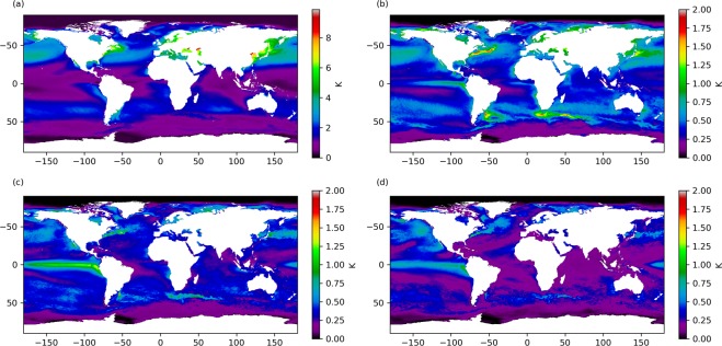
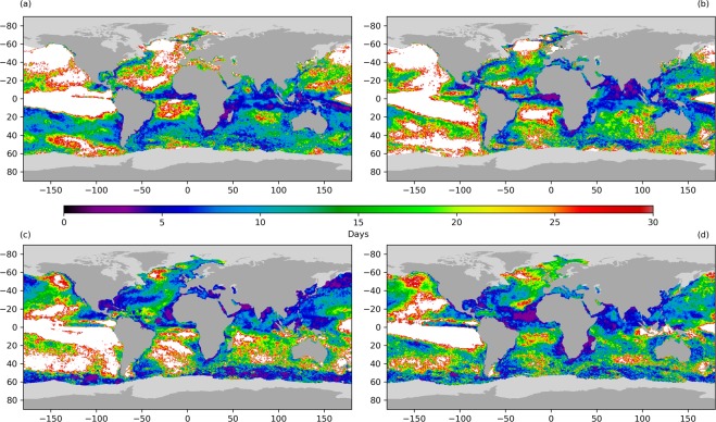
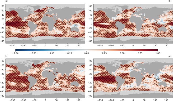
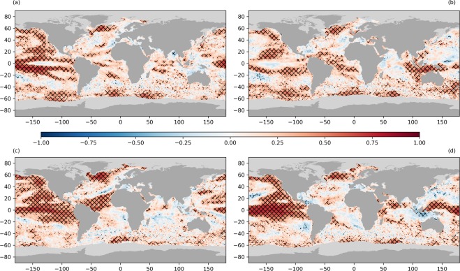
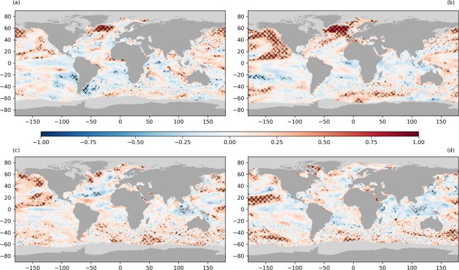
![Figure 7 (a) Uncertainty in the Theil-Sen slope fit82 of the sea-surface temperature anomaly (SSTA) trend between 1981–2018 at 0.25 degree resolution. (b) Timeseries of SSTA uncertainties between 1981–2018 for global data (black), the Atlantic Meridional Variability Region [0–65 N, 75–7.5 W30 (blue), the Nino 3.4 region [5N-5S, 170–120 W31 (red) and the NE Pacific warm waters [32–54 N, 165–138 W32 (cyan). Uncertainties in decadal tendencies (degrees kelvin per decade) calculated from data for (c) 1981–1989, (d) 1990–1999, (e) 2000–2009 and (f) 2010–2018 are at one degree resolution. Note that the colour scale is different (0–1.5 K) for decadal panels (c–f) than for the full-period figure (a, 0–0.4 K).](/paper-figures/a24806001dea420e89e00c8e86040af0/tendencies-variability-and-persistence-of-sea-surface-temperature-anomalies-figure-7.jpg)
Verification
Claims the paper makes
69 Own result · 21 No full text of the sources · 21 Own interpretation · 19 Partly supported · 14 No basis given · 7 Sources not found · 5 Supported · 4 Supported so far · 4 Own method · 2 Couldn’t confirm · accuracy not yet measured
The cited sources support only part of this claim — read each source’s verdict below.
In the paper
“The AMV region shows a step change in the SSTA centred on 1995, corresponding to the change to a positive phase of the AMV30.”
§ Tendencies, variability and persistence of sea surface temperature anomalies > Results > SST Trends
What the sources say
- Partly supportedcites [30] Sutton, R. T. et al. Atlantic Multidecadal Variability and the UK ACSIS Program. BAMS 415–425 (2018). sourceExperimental — accuracy not yet measured
The 'Observed Characteristics of AMV' section (page unavailable) places the cool phase at approximately 1965–95 and the warm phase from 2000 onward, and explicitly describes a 1990s shift to positive AMV. It does not describe a step change in sea-surface-temperature anomalies centred on 1995, so that characterization is not established by the text. (LLM, conf=0.83)
plaincorrelational- Asserted: passes — The authors put it forward as true.
- Checkable: passes — It can be checked against evidence.
- Load-bearing: unclear — It is unclear whether the paper’s conclusions depend on it.
- Based: passes — The paper gives a reason why it holds.
- Partly supported
The cited sources support only part of this claim — read each source’s verdict below.
In the paper
“Regional studies have demonstrated the independence of the re-emergence signal from ENSO variability15 with the strongest re-emergence signals in the NW Pacific, NW Atlantic and Southern Ocean16–18.”
§ Tendencies, variability and persistence of sea surface temperature anomalies > Introduction
What the sources say
- Partly supportedcites [15] Zhao, X. & Li, J. Winter-to-Winter Recurrence of Sea Surface Temperature Anomalies in the Northern Hemisphere. Journal of Climate 32, 3835–3854 (2010). sourceExperimental — accuracy not yet measured
The Spatiotemporal distribution of the SSTA WWR section (page unavailable) reports recurrence across much of the North Pacific and North Atlantic, including the northwestern Pacific. It does not identify these as the strongest re-emergence signals or assess the Southern Ocean; the study is limited to the Northern Hemisphere. (LLM, conf=0.86)
- Not checked — no full text of the sourcecites [16] de Coetlogon, G. & Frankignoul, C. The Persistence of Winter Sea Surface Temperature in the North Atlantic. Journal of Climate 16, 1364–1377 (2002). source
- Not checked — no full text of the sourcecites [17] Timlin, M. S., Alexander, M. A. & Deser, C. On the Reemergence of North Atlantic SST Anomalies. Journal of Climate 15, 2707–2712 (2002). source
- Not checked — no full text of the sourcecites [18] Alexander, M. A., Deser, C. & Timlin, M. S. The Reemergence of SST Anomalies in the North Pacific Ocean. Journal of Climate 12, 2419–2433 (1999). source
boostedcorrelational- Asserted: passes — The authors put it forward as true.
- Checkable: passes — It can be checked against evidence.
- Load-bearing: unclear — It is unclear whether the paper’s conclusions depend on it.
- Based: passes — The paper gives a reason why it holds.
- Partly supported
The cited sources support only part of this claim — read each source’s verdict below.
In the paper
“This dataset is to the maximum degree possible independent of in-situ observations2.”
§ Tendencies, variability and persistence of sea surface temperature anomalies > Introduction
What the sources say
- Partly supportedcites [2] Merchant, C. J. et al. Satellite-based time-series of sea-surface temperature since 1981 for climate applications. Scientific Data 6, https://doi.org/10.1038/s41597-019-0236-x (2019). sourceExperimental — accuracy not yet measured
The Background & Summary says the dataset’s objective is to be as independent of in-situ observations as possible, and that a high degree of independence was achieved from 1995 onward. It also says in-situ SSTs were needed as a calibration reference for 1981–1995, when independence was lost to a significant degree. The claim presents the objective as a property of the dataset without that time-period qualification. (LLM, conf=0.88)
hedged- Asserted: passes — The authors put it forward as true.
- Checkable: passes — It can be checked against evidence.
- Load-bearing: passes — The paper’s conclusions depend on it.
- Based: passes — The paper gives a reason why it holds.
- Partly supported
The sources with a verdict support this claim; the rest weren’t checked yet, have no full text we could read, or their verdicts aren’t rated yet.
In the paper
“Regions characterised by a strong seasonal variation in MLD may also display the phenomenon of re-emergence of winter-to-winter SSTA9–13.”
§ Tendencies, variability and persistence of sea surface temperature anomalies > Introduction
What the sources say
- Not checked — no full text of the sourcecites [9] Byju, P., Dommenget, D. & Alexander, M. A. Widespread reemergence of sea surface temperature anomalies in the global oceans, including tropical regions forced by reemerging winds. Geophysical Research Letters, https://doi.org/10.1029/2018GL079137 7683–7691 (2018). source
- Supportedcites [10] Hanawa, K. & Sugimoto, S. ‘Reemergence’ areas of winter sea surface temperature anomalies in the world’s oceans. Geophysical Research Letters 31, https://doi.org/10.1029/2004GL019904 (2004). source
Section 3 ([11]) reports that all seven reemergence areas have large seasonal variation in mixed-layer depth. The Summary and Remarks ([15]) specifies that winter SST anomalies reemerged the next winter in five of those areas; the other two showed fall reemergence. The claim’s “may” accurately allows for that distinction. (LLM, conf=0.93)
- Not checked — no full text of the sourcecites [11] Alexander, M. A. & Deser, C. A Mechanism for the Recurrence of Wintertime Midlatitude SST anomalies. Journal of Physical Oceanography 25, 122–135 (1994). source
- Not checked — no full text of the sourcecites [12] Alexander, M. A., Timlin, M. S. & James, D. S. Winter-to-winter recurrence of sea surface temperature, salinity and mixed layer depth anomalies. Process in Oceanography 49, 41–61 (2001). source
- Not checked — no full text of the sourcecites [13] Namias, J. & Born, R. M. Temporal Coherence in North Pacific Sea-Surface Temperature Patterns. Journal of Geophysical Research 75, 5952–5955 (1970). source
hedgedconditional- Asserted: passes — The authors put it forward as true.
- Checkable: passes — It can be checked against evidence.
- Load-bearing: unclear — It is unclear whether the paper’s conclusions depend on it.
- Based: passes — The paper gives a reason why it holds.
The cited sources support only part of this claim — read each source’s verdict below.
In the paper
“The NE Pacific warm anomaly of 2014–2016 is markedly stronger (in this location) than any previous period in the dataset and is attributed to strong, persistent, positive sea-level pressure anomalies32.”
§ Tendencies, variability and persistence of sea surface temperature anomalies > Results > SST Trends
What the sources say
- Partly supportedcites [32] Bond, N. A., Cronin, M. F., Freeland, H. & Mantua, N. Causes and impacts of the 2014 warm anomaly in the NE Pacific. Geophysical Research Letters 3414–3420 (2015). sourceExperimental — accuracy not yet measured
The Introduction says the February 2014 temperature anomalies were the greatest observed in the region for that month since at least the 1980s. The Abstract attributes the anomaly to an unusually strong, persistent high-pressure pattern. The paper does not establish that the entire 2014–2016 anomaly was stronger than every previous period in the citing document’s dataset; its reported observations extend only into 2015. (LLM, conf=0.88)
boosted- Asserted: passes — The authors put it forward as true.
- Checkable: passes — It can be checked against evidence.
- Load-bearing: unclear — It is unclear whether the paper’s conclusions depend on it.
- Based: passes — The paper gives a reason why it holds.
- Partly supported
The cited sources support only part of this claim — read each source’s verdict below.
In the paper
“The dataset is strengthened with respect to other analysis products by the inclusion of data from the Along-Track Scanning Radiometer instruments, designed specifically to retrieve surface temperature rather than for more general meteorological applications.”
§ Tendencies, variability and persistence of sea surface temperature anomalies > Introduction
What the sources say
- Partly supportedcites [2] Merchant, C. J. et al. Satellite-based time-series of sea-surface temperature since 1981 for climate applications. Scientific Data 6, https://doi.org/10.1038/s41597-019-0236-x (2019). sourceExperimental — accuracy not yet measured
The Background & Summary says the SST CCI record uses ATSR sensors as calibration references to achieve a distinctive degree of independence from in situ observations. The Methods’ retrieval section also describes an advantage of ATSR’s dual-view observations over AVHRR’s single-view observations. These passages support ATSR as a strength of the dataset, but do not establish that it is stronger than other analysis products or state that ATSR was designed specifically for surface-temperature retrieval rather than general meteorology. (LLM, conf=0.82)
plaindirect- Asserted: passes — The authors put it forward as true.
- Checkable: passes — It can be checked against evidence.
- Load-bearing: unclear — It is unclear whether the paper’s conclusions depend on it.
- Based: passes — The paper gives a reason why it holds.
- Partly supported
The cited sources support only part of this claim — read each source’s verdict below.
In the paper
“The NE Pacific warm anomaly of 2014–2016 is markedly stronger (in this location) than any previous period in the dataset and is attributed to strong, persistent, positive sea-level pressure anomalies32.”
§ Tendencies, variability and persistence of sea surface temperature anomalies > Results > SST Trends
What the sources say
- Partly supportedcites [32] Bond, N. A., Cronin, M. F., Freeland, H. & Mantua, N. Causes and impacts of the 2014 warm anomaly in the NE Pacific. Geophysical Research Letters 3414–3420 (2015). sourceExperimental — accuracy not yet measured
The Abstract and Final Remarks attribute the winter 2013–2014 NE Pacific warming to an unusually strong, persistent pattern of positive sea-level pressure anomalies. The paper says warm sea-surface temperatures persisted through March 2015, but does not establish that this explanation applies to the full 2014–2016 period. (LLM, conf=0.87)
plaindirect- Asserted: passes — The authors put it forward as true.
- Checkable: passes — It can be checked against evidence.
- Load-bearing: passes — The paper’s conclusions depend on it.
- Based: passes — The paper gives a reason why it holds.
- Partly supported
The cited sources that could be checked couldn’t confirm or dispute this claim.
In the paper
“In the 2010’s we observe a distinctive tripole signature in the SSTA trends of the North Atlantic, associated with the mixed layer response to the NAO44.”
§ Tendencies, variability and persistence of sea surface temperature anomalies > Results > SST Trends
What the sources say
- Could not verifycites [44] Sutton, R. T., Norton, W. A. & Jewson, S. P. The North Atlantic Oscillation - What Role for the Ocean? Atmospheric Science Letters 1, 89–100 (2001). sourceExperimental — accuracy not yet measured
The discussion-meeting report (page not supplied) mentions sea-surface temperature only as an example of imposed zonal asymmetry. Searches of our copy for the North Atlantic tripole, 2010s SSTA trends, the NAO, and mixed-layer response found no passage addressing the attributed claim. (LLM, conf=0.77)
plaincorrelational- Asserted: passes — The authors put it forward as true.
- Checkable: passes — It can be checked against evidence.
- Load-bearing: unclear — It is unclear whether the paper’s conclusions depend on it.
- Based: passes — The paper gives a reason why it holds.
- Could not verify
The cited sources support only part of this claim — read each source’s verdict below.
In the paper
“This is an artefact of the SST data, where the retrieval is not robust to high concentrations of desert dust.”
§ Tendencies, variability and persistence of sea surface temperature anomalies > Results > SST Persistence
What the sources say
- Partly supportedcites [2] Merchant, C. J. et al. Satellite-based time-series of sea-surface temperature since 1981 for climate applications. Scientific Data 6, https://doi.org/10.1038/s41597-019-0236-x (2019). sourceExperimental — accuracy not yet measured
The Usage Notes (Fitness-for-purpose assessment) identify intermittent desert-dust-related biases in AVHRR SSTs in the northeast tropical Atlantic, supporting the proposed data-artefact mechanism. The paper does not establish that the specific short-term SSTA persistence west of Africa is caused by that bias, and it says ATSR-series sensors are much less sensitive to dust. (LLM, conf=0.84)
- Not checked — no full text of the sourcecites [61] Corlett, G. K. et al. The accuracy of SST retrievals from AATSR: An initial assessment through geophysical validation against in situ radiometers, buoys and other SST data sets. Advances in Space Research 37, 764–769 (2006). source
- Partly supportedcites [62] Reynolds, R. W., Gentemann, C. L. & Corlett, G. C. Evaluation of AATSR and TMI Satellite SST Data. Journal of Climate 23, 152–165 (2009). sourceExperimental — accuracy not yet measured
Section 3 (page unavailable) reports that Saharan dust aerosols may cause cold biases in infrared SST retrievals in the tropical Atlantic, supporting the concern about dust-sensitive data. It does not identify the cited short-term SSTA persistence as an artefact, and it says microwave retrievals are unaffected by aerosols while AATSR can compensate for them. (LLM, conf=0.84)
plaindirect- Asserted: passes — The authors put it forward as true.
- Checkable: passes — It can be checked against evidence.
- Load-bearing: passes — The paper’s conclusions depend on it.
- Based: passes — The paper gives a reason why it holds.
- Partly supported
The cited sources support only part of this claim — read each source’s verdict below.
In the paper
“Where dust events are not flagged as cloud in the retrieval, they tend to bias the retrieved SST cold2,61,62 and can cause an artificial timescale in the SSTA correlation, which then appears as short-term SSTA persistence.”
§ Tendencies, variability and persistence of sea surface temperature anomalies > Results > SST Persistence
What the sources say
- Supportedcites [2] Merchant, C. J. et al. Satellite-based time-series of sea-surface temperature since 1981 for climate applications. Scientific Data 6, https://doi.org/10.1038/s41597-019-0236-x (2019). source
The Usage Notes section says unscreened, unadjusted desert dust events cause intermittent negative biases in retrieved AVHRR SSTs. The Methods section also notes that dust-affected SSTs can pass quality screening without their aerosol bias being accounted for. (LLM, conf=0.94)
- Not checked — no full text of the sourcecites [61] Corlett, G. K. et al. The accuracy of SST retrievals from AATSR: An initial assessment through geophysical validation against in situ radiometers, buoys and other SST data sets. Advances in Space Research 37, 764–769 (2006). source
- Partly supportedcites [62] Reynolds, R. W., Gentemann, C. L. & Corlett, G. C. Evaluation of AATSR and TMI Satellite SST Data. Journal of Climate 23, 152–165 (2009). sourceExperimental — accuracy not yet measured
Section 3, “Data comparisons,” says Saharan dust aerosols may bias infrared SST retrievals cold and shows negative biases in AVHRR retrievals. It does not establish the claim’s condition that dust events were not flagged as cloud; it also notes that AATSR can compensate for aerosols and may instead show a small warm bias. The cited claim here is the cold-bias clause, not the sentence’s separate assertion about SSTA persistence. (LLM, conf=0.84)
plainconditional- Asserted: passes — The authors put it forward as true.
- Checkable: passes — It can be checked against evidence.
- Load-bearing: passes — The paper’s conclusions depend on it.
- Based: passes — The paper gives a reason why it holds.
- Supported
- It may state two separate claims as one. 49
- Probably not a substantial claim. 13
- The quote only partly states this claim. 1
Every source the paper cites for this claim was checked and supports it.
In the paper
“Changes in the AMV are coupled with the North Atlantic Oscillation and Atlantic Meridional Overturning Circulation (AMOC), with a positive phase of the AMV associated with warmer SSTs30.”
§ Tendencies, variability and persistence of sea surface temperature anomalies > Results > SST Trends
What the sources say
- Supportedcites [30] Sutton, R. T. et al. Atlantic Multidecadal Variability and the UK ACSIS Program. BAMS 415–425 (2018). source
The AMV MECHANISMS section describes interactions among the NAO, AMOC, and AMV. The figure description in CONCLUDING REMARKS identifies warmer SSTs with positive AMV. Page numbers are not provided in the supplied passages. (LLM, conf=0.94)
plaincorrelational- Asserted: passes — The authors put it forward as true.
- Checkable: passes — It can be checked against evidence.
- Load-bearing: unclear — It is unclear whether the paper’s conclusions depend on it.
- Based: passes — The paper gives a reason why it holds.
It may state two separate claims as one.
- Supported
The cited sources support only part of this claim — read each source’s verdict below.
In the paper
“In turn, ENSO state influences SSTA persistence in the Indian Ocean, where SSTA variability is comparatively small7.”
§ Tendencies, variability and persistence of sea surface temperature anomalies > Introduction
What the sources say
- Partly supportedcites [7] Ding, R. & Li, J. Influences of ENSO Teleconnection on the Persistence of Sea Surface Temperature in the Tropical Indian Ocean. Journal of Climate 25, 8177–8195 (2012). sourceExperimental — accuracy not yet measured
The Summary (page unavailable) reports that SSTA persistence barriers in parts of the tropical Indian Ocean weaken or disappear during weak or normal ENSO conditions, supporting the claim that ENSO state influences persistence. The paper does not establish that Indian Ocean SSTA variability is comparatively small overall; Section 3 (page unavailable) describes very small anomalies only for normal ENSO cases. (LLM, conf=0.85)
plaindirect- Asserted: passes — The authors put it forward as true.
- Checkable: passes — It can be checked against evidence.
- Load-bearing: unclear — It is unclear whether the paper’s conclusions depend on it.
- Based: passes — The paper gives a reason why it holds.
It may state two separate claims as one.
- Partly supported
The cited sources support only part of this claim — read each source’s verdict below.
In the paper
“The North-East Pacific between 45–55 N and 130–150 W is of interest due to the significant warm anomaly in the SST seen between 2014–2016, which had impacts on fisheries and regional weather32.”
§ Tendencies, variability and persistence of sea surface temperature anomalies > Introduction
What the sources say
- Partly supportedcites [32] Bond, N. A., Cronin, M. F., Freeland, H. & Mantua, N. Causes and impacts of the 2014 warm anomaly in the NE Pacific. Geophysical Research Letters 3414–3420 (2015). sourceExperimental — accuracy not yet measured
The Abstract says the anomaly affected downwind air temperatures in Washington state, and Biological Impacts describes unusual salmon movements and tuna catches in 2014. The Introduction reports anomalously warm SSTs persisting through March 2015; this paper does not establish the claimed 2014–2016 span. Page numbers are unavailable in our copy. (LLM, conf=0.88)
plaindirect- Asserted: passes — The authors put it forward as true.
- Checkable: passes — It can be checked against evidence.
- Load-bearing: fails — The paper’s conclusions may not depend on it.
- Based: passes — The paper gives a reason why it holds.
Probably not a substantial claim. The paper’s conclusions may not depend on it.
- Partly supported
Every source the paper cites for this claim was checked and supports it.
In the paper
“Western boundary currents (WBCs) are turbulent areas of water characterised by strong ocean-atmosphere interaction, poleward heat transport and ocean-atmosphere heat exchange20.”
§ Tendencies, variability and persistence of sea surface temperature anomalies > Introduction
What the sources say
- Supportedcites [20] Kwon, Y.-O. et al. Role of the Gulf Stream and Kuroshio-Oyashio Systems in Large-Scale Atmosphere-Ocean Interaction: A Review. Journal of Climate 23, 3249–3281 (2010). source
The Introduction describes exceptionally strong atmosphere–ocean interaction over western boundary currents and their extensions. It also describes poleward ocean heat transport and heat transfer to the atmosphere concentrated near these currents; the Abstract identifies mesoscale eddies as important in these regions, consistent with the description of turbulent waters. (LLM, conf=0.90)
plaincorrelational- Asserted: passes — The authors put it forward as true.
- Checkable: passes — It can be checked against evidence.
- Load-bearing: fails — The paper’s conclusions may not depend on it.
- Based: passes — The paper gives a reason why it holds.
Probably not a substantial claim. The paper’s conclusions may not depend on it. It may state two separate claims as one.
- Supported
The sources with a verdict support this claim; the rest weren’t checked yet, have no full text we could read, or their verdicts aren’t rated yet.
In the paper
“Winter SST anomalies persist at depth during the summer months below the shallow mixed layer, reemerging in the SSTA the following winter as the summer seasonal thermocline is eroded.”
§ Tendencies, variability and persistence of sea surface temperature anomalies > Introduction
What the sources say
- Not checked — no full text of the sourcecites [9] Byju, P., Dommenget, D. & Alexander, M. A. Widespread reemergence of sea surface temperature anomalies in the global oceans, including tropical regions forced by reemerging winds. Geophysical Research Letters, https://doi.org/10.1029/2018GL079137 7683–7691 (2018). source
- Supportedcites [10] Hanawa, K. & Sugimoto, S. ‘Reemergence’ areas of winter sea surface temperature anomalies in the world’s oceans. Geophysical Research Letters 31, https://doi.org/10.1029/2004GL019904 (2004). source
Section 3 ([12]) describes anomalous water formed in the deep winter mixed layer being capped by the shallow seasonal thermocline during the warming season, then entrained as the mixed layer deepens in the next cooling season. Section 4 ([13]) reports that winter SST anomalies reemerge the next winter in several regions, although in two others they reemerge in early fall and are subsequently refreshed. (LLM, conf=0.91)
- Not checked — no full text of the sourcecites [11] Alexander, M. A. & Deser, C. A Mechanism for the Recurrence of Wintertime Midlatitude SST anomalies. Journal of Physical Oceanography 25, 122–135 (1994). source
- Not checked — no full text of the sourcecites [12] Alexander, M. A., Timlin, M. S. & James, D. S. Winter-to-winter recurrence of sea surface temperature, salinity and mixed layer depth anomalies. Process in Oceanography 49, 41–61 (2001). source
- Not checked — no full text of the sourcecites [13] Namias, J. & Born, R. M. Temporal Coherence in North Pacific Sea-Surface Temperature Patterns. Journal of Geophysical Research 75, 5952–5955 (1970). source
plaindirect- Asserted: passes — The authors put it forward as true.
- Checkable: passes — It can be checked against evidence.
- Load-bearing: passes — The paper’s conclusions depend on it.
- Based: passes — The paper gives a reason why it holds.
It may state two separate claims as one.
Every source the paper cites for this claim was checked and supports it.
In the paper
“In the sub-polar gyre we see significant warming in the 1990’s and cooling in the 2010’s whilst the reverse is true for the north-east Pacific in the region of the recent warm anomaly32.”
§ Tendencies, variability and persistence of sea surface temperature anomalies > Results > SST Variability
What the sources say
- Supportedcites [32] Bond, N. A., Cronin, M. F., Freeland, H. & Mantua, N. Causes and impacts of the 2014 warm anomaly in the NE Pacific. Geophysical Research Letters 3414–3420 (2015). source
The citation follows “the recent warm anomaly,” and Bond et al. identify and locate that anomaly in the Introduction. The preceding decadal comparison is framed as the citing authors’ own observation, not as a finding attributed to Bond et al. (LLM, conf=0.87)
plaincorrelational- Asserted: passes — The authors put it forward as true.
- Checkable: passes — It can be checked against evidence.
- Load-bearing: unclear — It is unclear whether the paper’s conclusions depend on it.
- Based: passes — The paper gives a reason why it holds.
It may state two separate claims as one.
- Supported
Every source the paper cites for this claim was checked and supports it.
In the paper
“It is also consistent with the subsurface temperature trends (warming from the mid-80’s to 2006 and cooling thereafter), with a time-lag between subsurface temperatures and subsequent surface temperature signals41.”
§ Tendencies, variability and persistence of sea surface temperature anomalies > Results > SST Trends
What the sources say
- Supportedcites [41] Ruiz-Barradas, A., Chafik, L., Nigam, S. & Hakkinen, S. Recent subsurface North Atlantic cooling trend in context of Atlantic decadal-to-multidecadal variability. Tellus 70 (2018). source
The Results section reports a 1985–2005 warming trend followed by post-2006 subsurface cooling. It also says subpolar gyre SST and heat-content anomalies peaked in 2006–2007 before cooling, and that surface thermal variations there lag subsurface subtropical variations by about five years. No page number is available in our copy. (LLM, conf=0.90)
plaincorrelational- Asserted: passes — The authors put it forward as true.
- Checkable: passes — It can be checked against evidence.
- Load-bearing: unclear — It is unclear whether the paper’s conclusions depend on it.
- Based: passes — The paper gives a reason why it holds.
It may state two separate claims as one.
- Supported
The cited sources support only part of this claim — read each source’s verdict below.
In the paper
“The “global warming hiatus”47,48, is seen in Fig. 1e, referring to a decade (2000 to 2009) during which global mean SSTA changed less than in the previous or subsequent decade.”
§ Tendencies, variability and persistence of sea surface temperature anomalies > Results > SST Trends
What the sources say
- Partly supportedcites [47] Trenberth, K. E. & Fasullo, J. T. An apparent hiatus in global warming? Earth’s Future 1, 19–32 (2013). sourceExperimental — accuracy not yet measured
The Introduction (page unavailable) calls the slowed rise in global mean temperature during the 2000s a “hiatus or plateau.” The paper discusses global surface temperature, not the claimed decade-by-decade comparison of global mean sea-surface temperature anomalies; published in 2013, it does not establish how 2000–2009 compares with the subsequent decade. (LLM, conf=0.86)
- Partly supportedcites [48] Fyfe, J. C. et al. Making sense of the early-2000s warming slowdown. Nature Climate Change 6, 224–228 (2016). sourceExperimental — accuracy not yet measured
The Concluding remarks say that global mean surface temperature warmed more slowly in the early 21st century than in the previous few decades. But the Figure 1 caption starts the slowdown in 2001, and the paper discusses it through 2014; it does not define the hiatus as 2000–2009 or establish the claimed comparison with the subsequent decade in global mean sea-surface temperature anomaly (SSTA). (LLM, conf=0.87)
plain- Asserted: passes — The authors put it forward as true.
- Checkable: passes — It can be checked against evidence.
- Load-bearing: passes — The paper’s conclusions depend on it.
- Based: passes — The paper gives a reason why it holds.
Probably not a substantial claim.
- Partly supported
The cited sources support only part of this claim — read each source’s verdict below.
In the paper
“SSTA variability in this region has been linked to the AMOC, which was moving into a positive phase in the 1990’s (warming trend in SSTAs), peaking in the 2000’s and then declining in the 2010’s (cooling trend in SSTAs)37–40.”
§ Tendencies, variability and persistence of sea surface temperature anomalies > Results > SST Trends
What the sources say
- Partly supportedcites [37] Reverdin, G. et al. North Atlantic extratropical and subpolar gyre variability during the last 120 years: a gridded dataset of surface temperature, salinity, and density. Part 1: Dataset validation and RMS variability. Ocean Dynamics 69, 385–403 (2019). sourceExperimental — accuracy not yet measured
The Introduction (page unavailable) links subpolar-gyre surface properties to the AMOC, but says the connection between surface changes and the AMOC remains under discussion. The passages do not establish that the AMOC entered a positive phase in the 1990s, peaked in the 2000s, or declined in the 2010s; the paper’s SST observations do not by themselves establish that AMOC chronology. (LLM, conf=0.84)
- Not checked — no full text of the sourcecites [38] Deser, C., Alexander, M., Xie, S.-P. & Phillips, A. S. Sea Surface Temperature Variability: Patterns and Mechanisms. Annual Review of Marine Science 2, 115–43 (2010). source
- Not checked — no full text of the sourcecites [39] Chen, X. & Tung, K. K. Global surface warming enhanced by weak Atlantic overturning circulation. Nature 559, 387–391 (2018). source
- Partly supportedcites [40] Robson, J., Ortega, P. & Sutton, R. A reversal of climatic trends in the North Atlantic since 2005. Nature Geoscience 9, 513–517 (2016). sourceExperimental — accuracy not yet measured
The Abstract links rapid subpolar-gyre warming in the mid-1990s to a strengthening AMOC and reports cooling since 2005 consistent with weaker ocean circulation. It does not establish an AMOC peak in the 2000s; instead, it says measurements suggest circulation strength has declined since the mid-1990s. (LLM, conf=0.85)
plaincorrelational- Asserted: passes — The authors put it forward as true.
- Checkable: passes — It can be checked against evidence.
- Load-bearing: passes — The paper’s conclusions depend on it.
- Based: passes — The paper gives a reason why it holds.
It may state two separate claims as one.
- Partly supported
The cited sources support only part of this claim — read each source’s verdict below.
In the paper
“The areas with the strongest warming trends during 2010–2018 are the North and East Pacific, the trend being driven by the warm anomalies observed here between 2014–201632,49.”
§ Tendencies, variability and persistence of sea surface temperature anomalies > Results > SST Trends
What the sources say
- Partly supportedcites [32] Bond, N. A., Cronin, M. F., Freeland, H. & Mantua, N. Causes and impacts of the 2014 warm anomaly in the NE Pacific. Geophysical Research Letters 3414–3420 (2015). sourceExperimental — accuracy not yet measured
The Introduction (page not available) documents unusually warm NE Pacific waters in 2014 and says anomalously warm sea surface temperatures persisted through March 2015. It does not assess which regions had the strongest warming trends in 2010–2018 or establish that anomalies through 2016 drove those trends. (LLM, conf=0.88)
- Not checked — no full text of the sourcecites [49] Gentemann, C. L., Fewings, M. R. & Garcia-Reyes, M. Satellite sea surface temperatures along the West Coast of the United States during the 2014-2016 northeast Pacific marine heatwave. Geophysical Research Letters 44, 312–319 (2017). source
plaindirect- Asserted: passes — The authors put it forward as true.
- Checkable: passes — It can be checked against evidence.
- Load-bearing: passes — The paper’s conclusions depend on it.
- Based: passes — The paper gives a reason why it holds.
It may state two separate claims as one.
- Partly supported
The cited sources support only part of this claim — read each source’s verdict below.
In the paper
“Decadal temperature trends here are consistent in sign with the sub-polar gyre, but much smaller in magnitude with an overall neutral trend between 1981–2018, also seen in-situ data records37.”
§ Tendencies, variability and persistence of sea surface temperature anomalies > Results > SST Trends
What the sources say
- Partly supportedcites [37] Reverdin, G. et al. North Atlantic extratropical and subpolar gyre variability during the last 120 years: a gridded dataset of surface temperature, salinity, and density. Part 1: Dataset validation and RMS variability. Ocean Dynamics 69, 385–403 (2019). sourceExperimental — accuracy not yet measured
Section 3.3 (page unavailable) reports good agreement between two surface-temperature records in the subpolar gyre and regions farther south. Section 4 (page unavailable) reports spatially varying temperature trends, including cooling near West Greenland and the central Labrador Sea. Neither passage establishes a smaller trend south of Greenland or an overall neutral trend for 1981–2018; the paper’s reported trend analysis ends in 2015. (LLM, conf=0.82)
plaincorrelational- Asserted: passes — The authors put it forward as true.
- Checkable: passes — It can be checked against evidence.
- Load-bearing: unclear — It is unclear whether the paper’s conclusions depend on it.
- Based: passes — The paper gives a reason why it holds.
It may state two separate claims as one.
- Partly supported
The cited sources support only part of this claim — read each source’s verdict below.
In the paper
“Where dust events are not flagged as cloud in the retrieval, they tend to bias the retrieved SST cold2,61,62 and can cause an artificial timescale in the SSTA correlation, which then appears as short-term SSTA persistence.”
§ Tendencies, variability and persistence of sea surface temperature anomalies > Results > SST Persistence
What the sources say
- Partly supportedcites [2] Merchant, C. J. et al. Satellite-based time-series of sea-surface temperature since 1981 for climate applications. Scientific Data 6, https://doi.org/10.1038/s41597-019-0236-x (2019). sourceExperimental — accuracy not yet measured
The Usage Notes (Fitness-for-purpose assessment) say that unscreened desert dust causes intermittent cold biases in retrieved SST and an exaggerated trend in SST anomalies. They do not say that dust creates an artificial timescale in SSTA correlation or apparent short-term persistence. (LLM, conf=0.84)
- Not checked — no full text of the sourcecites [61] Corlett, G. K. et al. The accuracy of SST retrievals from AATSR: An initial assessment through geophysical validation against in situ radiometers, buoys and other SST data sets. Advances in Space Research 37, 764–769 (2006). source
- Partly supportedcites [62] Reynolds, R. W., Gentemann, C. L. & Corlett, G. C. Evaluation of AATSR and TMI Satellite SST Data. Journal of Climate 23, 152–165 (2009). sourceExperimental — accuracy not yet measured
Section 3 (Data comparisons; page unavailable) reports that Saharan dust aerosols may bias infrared SST retrievals cold, with negative biases observed in AVHRR data. It does not establish that dust events escape cloud flagging or that they create an artificial timescale in SSTA correlations or apparent short-term persistence. (LLM, conf=0.86)
plaindirect- Asserted: passes — The authors put it forward as true.
- Checkable: passes — It can be checked against evidence.
- Load-bearing: passes — The paper’s conclusions depend on it.
- Based: passes — The paper gives a reason why it holds.
It may state two separate claims as one.
- Partly supported
The sources with a verdict support this claim; the rest weren’t checked yet, have no full text we could read, or their verdicts aren’t rated yet.
In the paper
“This is typically characterised as winter-to-winter re-emergence although the time lag can be variable, ranging from 7–13 months15, and is usually seen in the mid-latitudes12,15–19.”
§ Tendencies, variability and persistence of sea surface temperature anomalies > Results > SST Persistence
What the sources say
- Supportedcites [15] Zhao, X. & Li, J. Winter-to-Winter Recurrence of Sea Surface Temperature Anomalies in the Northern Hemisphere. Journal of Climate 32, 3835–3854 (2010). source
The Introduction describes winter-to-winter recurrence of midlatitude sea-surface temperature anomalies. The Spatiotemporal Distribution section reports recurrence maxima around 7–8 months in some regions and winter recurrence at 11–13 months in others, supporting the stated variable lag. The paper also finds subtropical recurrence, which does not conflict with the claim that recurrence is usually seen in midlatitudes. (LLM, conf=0.88)
- Not checked — no full text of the sourcecites [12] Alexander, M. A., Timlin, M. S. & James, D. S. Winter-to-winter recurrence of sea surface temperature, salinity and mixed layer depth anomalies. Process in Oceanography 49, 41–61 (2001). source
- Not checked — no full text of the sourcecites [16] de Coetlogon, G. & Frankignoul, C. The Persistence of Winter Sea Surface Temperature in the North Atlantic. Journal of Climate 16, 1364–1377 (2002). source
- Not checked — no full text of the sourcecites [17] Timlin, M. S., Alexander, M. A. & Deser, C. On the Reemergence of North Atlantic SST Anomalies. Journal of Climate 15, 2707–2712 (2002). source
- Not checked — no full text of the sourcecites [18] Alexander, M. A., Deser, C. & Timlin, M. S. The Reemergence of SST Anomalies in the North Pacific Ocean. Journal of Climate 12, 2419–2433 (1999). source
- Not checked — no full text of the sourcecites [19] Sugimoto, S. & Hanawa, K. Remote reemergence of areas of winter sea surface temperature anomalies in the north Pacific. Geophysical Research Letters 32 (2005). source
plaincorrelational- Asserted: passes — The authors put it forward as true.
- Checkable: passes — It can be checked against evidence.
- Load-bearing: unclear — It is unclear whether the paper’s conclusions depend on it.
- Based: passes — The paper gives a reason why it holds.
It may state two separate claims as one.
- Supported
The cited sources support only part of this claim — read each source’s verdict below.
In the paper
“The Pacific Decadal Oscillation (PDO) also transitioned from a positive to negative phase over the 1980’s-2000’s, becoming more neutral in the 2010’s.”
§ Tendencies, variability and persistence of sea surface temperature anomalies > Discussion
What the sources say
- Not checked — no full text of the sourcecites [35] Falvey, M. & Garreaud, R. D. Regional cooling in a warming world: Recent temperature trends in the southeast Pacific and along the west coast of subtropical South America (1979-2006). Journal of Geophysical Research 114 (2009). source
- Partly supportedcites [78] Meehl, G. A. et al. Sustained ocean changes contributed to sudden Antarctic sea ice retreat in late 2016. Nature Communications 10 (2019). sourceExperimental — accuracy not yet measured
The Introduction (page unavailable) describes a positive-to-negative shift across 1979–2000 and the post-2000 period, but it identifies the oscillation as the IPO, not the PDO. It also describes a transition toward a positive IPO phase in 2014–2016, rather than saying it became more neutral in the 2010s. (LLM, conf=0.84)
plain- Asserted: passes — The authors put it forward as true.
- Checkable: passes — It can be checked against evidence.
- Load-bearing: unclear — It is unclear whether the paper’s conclusions depend on it.
- Based: passes — The paper gives a reason why it holds.
It may state two separate claims as one.
The cited sources support only part of this claim — read each source’s verdict below.
In the paper
“Cooling in the Southern Pacific is consistent with the PDO becoming more negative (1980’s-2000’s) and warming consistent with a return towards a positive index (2010’s)35,78.”
§ Tendencies, variability and persistence of sea surface temperature anomalies > Discussion
What the sources say
- Not checked — no full text of the sourcecites [35] Falvey, M. & Garreaud, R. D. Regional cooling in a warming world: Recent temperature trends in the southeast Pacific and along the west coast of subtropical South America (1979-2006). Journal of Geophysical Research 114 (2009). source
- Partly supportedcites [78] Meehl, G. A. et al. Sustained ocean changes contributed to sudden Antarctic sea ice retreat in late 2016. Nature Communications 10 (2019). sourceExperimental — accuracy not yet measured
The Introduction (page not specified) links below-normal southern-latitude sea-surface temperatures to a negative interdecadal Pacific oscillation (IPO) and describes a possible transition toward a positive IPO in 2014–2016. But it places the negative phase in 2000–2014 and the positive phase in 1979–2000, contrary to the claim’s 1980s–2000s timing. It discusses the IPO, not the PDO. (LLM, conf=0.86)
plaincorrelational- Asserted: passes — The authors put it forward as true.
- Checkable: passes — It can be checked against evidence.
- Load-bearing: unclear — It is unclear whether the paper’s conclusions depend on it.
- Based: passes — The paper gives a reason why it holds.
It may state two separate claims as one.
The sources with a verdict support this claim; the rest weren’t checked yet, have no full text we could read, or their verdicts aren’t rated yet.
In the paper
“this may suggest that natural decadal variability is also important73,76, or that the timing of different response mechanisms in the models is not adequately resolved74,77.”
§ Tendencies, variability and persistence of sea surface temperature anomalies > Discussion
What the sources say
- Not matchedcites [73] Armour, K. C. & Bitz, C. M. Observed and projected trends in Antarctic sea ice. US CLIVAR Variations 13, 12–19 (2015).
Couldn’t be matched to a paper in Crossref, so it can’t be checked.
- Not checked — no full text of the sourcecites [76] Fan, T., Deser, C. & Schneider, D. P. Recent Antarctic sea ice trends in the context of Southern Ocean surface climate variations since 1950. Geophysical Research Letters 141, 2419–2426 (2014). source
- Supportedcites [74] Kostov, Y. et al. Fast and slow responses of Southern Ocean sea surface temperature to SAM in coupled climate models. Climate Dynamics 48, 1595–1609 (2017). source
This source is cited for the timing of response mechanisms, not for natural decadal variability. The Results report that a CMIP5 bias in inversion depth may make models overestimate how quickly subsurface warming reaches the mixed layer; the Discussion links model climatology to how quickly the response shifts from cooling to warming. Page numbers are unavailable in our copy. (LLM, conf=0.87)
- Supportedcites [77] Ferreira, D. & Marshall, J. Antarctic Ocean and Sea Ice Response to Ozone Depletion: A Two-Time-Scale Problem. Journal of Climate 28, 1206–1226 (2015). source
The citation is attached to the proposed explanation about model timing, not the separate suggestion about natural variability. The Conclusions report that the transition from cooling to warming is poorly constrained—20 years in one model versus 3–5 years in the other—and identify uncertain air–sea and ocean processes that affect it. The paper does not itself assess a failure of CMIP5 models to reproduce observed cooling. (LLM, conf=0.87)
hedgedconditional- Asserted: passes — The authors put it forward as true.
- Checkable: passes — It can be checked against evidence.
- Load-bearing: passes — The paper’s conclusions depend on it.
- Based: passes — The paper gives a reason why it holds.
It may state two separate claims as one.
- Not matched
Every source the paper cites for this claim was checked and supports it.
In the paper
“From the end of 2016 onwards, a sharp decrease in Antarctic sea-ice has also been observed78”
§ Tendencies, variability and persistence of sea surface temperature anomalies > Discussion
What the sources say
- Supportedcites [78] Meehl, G. A. et al. Sustained ocean changes contributed to sudden Antarctic sea ice retreat in late 2016. Nature Communications 10 (2019). source
The Introduction reports a sudden decrease in Antarctic sea ice in late 2016. The Discussion says reduced sea-ice extent persisted through winter 2018, supporting the claim that the retreat continued after 2016. (LLM, conf=0.94)
plain- Asserted: passes — The authors put it forward as true.
- Checkable: passes — It can be checked against evidence.
- Load-bearing: fails — The paper’s conclusions may not depend on it.
- Based: passes — The paper gives a reason why it holds.
Probably not a substantial claim. The paper’s conclusions may not depend on it.
- Supported
A result the paper reports from its own data — it cites no other source for it, so there is none to check. The quote shows it is in the paper.
In the paper
“The strongest warming trends are in the Northern Hemisphere close to the Arctic sea-ice boundary, in the Mediterranean, in the Black Sea and along the northern edge of the Northern Hemisphere western boundary currents (Gulf Stream and Kuroshio Extension).”
§ Tendencies, variability and persistence of sea surface temperature anomalies > Results > SST Trends
plain- Asserted: passes — The authors put it forward as true.
- Checkable: passes — It can be checked against evidence.
- Load-bearing: passes — The paper’s conclusions depend on it.
- Based: passes — The paper gives a reason why it holds.
It may state two separate claims as one.
A result the paper reports from its own data — it cites no other source for it, so there is none to check. The quote shows it is in the paper.
In the paper
“SSTA fluctuations in the Nino 3.4 region have a range of ~3–5 K, with positive SSTA’s associated with El-Nino events.”
§ Tendencies, variability and persistence of sea surface temperature anomalies > Results > SST Trends
plaincorrelational- Asserted: passes — The authors put it forward as true.
- Checkable: passes — It can be checked against evidence.
- Load-bearing: unclear — It is unclear whether the paper’s conclusions depend on it.
- Based: passes — The paper gives a reason why it holds.
It may state two separate claims as one.
A result the paper reports from its own data — it cites no other source for it, so there is none to check. The quote shows it is in the paper.
In the paper
“The median global short-term persistence length is 12 days in December, 14 days in March, 11 days in June and 12 days in September.”
§ Tendencies, variability and persistence of sea surface temperature anomalies > Results > SST Persistence
plain- Asserted: passes — The authors put it forward as true.
- Checkable: passes — It can be checked against evidence.
- Load-bearing: passes — The paper’s conclusions depend on it.
- Based: passes — The paper gives a reason why it holds.
It may state two separate claims as one.
A result the paper reports from its own data — it cites no other source for it, so there is none to check. The quote shows it is in the paper.
In the paper
“Short-term SSTA persistence is observed over 70.9, 71.0, 71.6 and 78.5% of the global oceans in each season respectively.”
§ Tendencies, variability and persistence of sea surface temperature anomalies > Results > SST Persistence
plaincorrelational- Asserted: passes — The authors put it forward as true.
- Checkable: passes — It can be checked against evidence.
- Load-bearing: passes — The paper’s conclusions depend on it.
- Based: passes — The paper gives a reason why it holds.
It may state two separate claims as one.
A result the paper reports from its own data — it cites no other source for it, so there is none to check. The quote shows it is in the paper.
In the paper
“Moreover, the localised trends in SSTA are in general significantly smaller than in other decades, with a standard deviation in the SSTA trends of 0.33 K in the 2000’s compared with 0.49–0.66 K for the other decades.”
§ Tendencies, variability and persistence of sea surface temperature anomalies > Results > SST Trends
plain- Asserted: passes — The authors put it forward as true.
- Checkable: passes — It can be checked against evidence.
- Load-bearing: passes — The paper’s conclusions depend on it.
- Based: passes — The paper gives a reason why it holds.
It may state two separate claims as one.
In the paper
“The cycle in the northern mid-latitudes is greater than that of the southern mid-latitudes51, with a mean standard deviation of 3.4 K for 30–50 N vs. 1.6 K for 30–50 S.”
§ Tendencies, variability and persistence of sea surface temperature anomalies > Results > SST Variability
What the sources say
- Not checked — no full text of the sourcecites [51] Casey, K. S. & Cornillon, P. A Comparision of Satellite and In Situ-Based Sea Surface Temperature Climatologies. Journal of Climate 12, 1848–1863 (1998). source
plaincorrelational- Asserted: passes — The authors put it forward as true.
- Checkable: passes — It can be checked against evidence.
- Load-bearing: unclear — It is unclear whether the paper’s conclusions depend on it.
- Based: passes — The paper gives a reason why it holds.
It may state two separate claims as one.
In the paper
“The warm anomaly maximum was observed in the offshore northerly region and along the west coast of the USA49.”
§ Tendencies, variability and persistence of sea surface temperature anomalies > Results > SST Trends
What the sources say
- Not checked — no full text of the sourcecites [49] Gentemann, C. L., Fewings, M. R. & Garcia-Reyes, M. Satellite sea surface temperatures along the West Coast of the United States during the 2014-2016 northeast Pacific marine heatwave. Geophysical Research Letters 44, 312–319 (2017). source
plain- Asserted: passes — The authors put it forward as true.
- Checkable: passes — It can be checked against evidence.
- Load-bearing: unclear — It is unclear whether the paper’s conclusions depend on it.
- Based: passes — The paper gives a reason why it holds.
It may state two separate claims as one.
A result the paper reports from its own data — it cites no other source for it, so there is none to check. The quote shows it is in the paper.
In the paper
“In the ENSO region the timeseries trend is also non-linear with a cooling in the 1980’s and 1990’s and a warming in the 2010’s following the hiatus period of the 2000’s.”
§ Tendencies, variability and persistence of sea surface temperature anomalies > Results > SST Variability
plain- Asserted: passes — The authors put it forward as true.
- Checkable: passes — It can be checked against evidence.
- Load-bearing: unclear — It is unclear whether the paper’s conclusions depend on it.
- Based: passes — The paper gives a reason why it holds.
It may state two separate claims as one.
The paper states this without a source or data behind it here, so there is nothing to check it against. The quote shows it is in the paper.
In the paper
“Temperature anomalies in the ENSO region of the tropical, eastern Pacific exhibit decadal variability - cooling in the 1980’s, warming close to the South American west coast in the 1990’s with cooling in the equatorial waters, weak warming in the 2000’s during the hiatus period, and a strong warming signal both close the the South American coast and in equatorial waters in the 2010’s.”
§ Tendencies, variability and persistence of sea surface temperature anomalies > Results > SST Trends
plaincorrelational- Asserted: passes — The authors put it forward as true.
- Checkable: passes — It can be checked against evidence.
- Load-bearing: passes — The paper’s conclusions depend on it.
- Based: passes — The paper gives a reason why it holds.
It may state two separate claims as one.
A result the paper reports from its own data — it cites no other source for it, so there is none to check. The quote shows it is in the paper.
In the paper
“We see that some SST variability in western boundary currents can be attributed to SST processes operating on those timescales, although this may be aliasing given the relatively short length of the timeseries.”
§ Tendencies, variability and persistence of sea surface temperature anomalies > Results > SST Variability
hedgedconditional- Asserted: passes — The authors put it forward as true.
- Checkable: passes — It can be checked against evidence.
- Load-bearing: unclear — It is unclear whether the paper’s conclusions depend on it.
- Based: passes — The paper gives a reason why it holds.
It may state two separate claims as one.
A result the paper reports from its own data — it cites no other source for it, so there is none to check. The quote shows it is in the paper.
In the paper
“In the ENSO region, SST power is dominated by SST processes on 1–5 year timescales, with a maximum SSTA variance of 1.9 K2.”
§ Tendencies, variability and persistence of sea surface temperature anomalies > Results > SST Variability
plaincorrelational- Asserted: passes — The authors put it forward as true.
- Checkable: passes — It can be checked against evidence.
- Load-bearing: unclear — It is unclear whether the paper’s conclusions depend on it.
- Based: passes — The paper gives a reason why it holds.
It may state two separate claims as one.
A result the paper reports from its own data — it cites no other source for it, so there is none to check. The quote shows it is in the paper.
In the paper
“The annual cycle is small (~1 K) at equatorial and very high latitudes, and is at a maximum at mid-latitudes.”
§ Tendencies, variability and persistence of sea surface temperature anomalies > Results > SST Variability
plaincorrelational- Asserted: passes — The authors put it forward as true.
- Checkable: passes — It can be checked against evidence.
- Load-bearing: unclear — It is unclear whether the paper’s conclusions depend on it.
- Based: passes — The paper gives a reason why it holds.
It may state two separate claims as one.
A result the paper reports from its own data — it cites no other source for it, so there is none to check. The quote shows it is in the paper.
In the paper
“There is considerable inter-decadal variation in within-decade temperature tendencies (Fig. 1c–f), which is particularly notable in the sub-Greenland gyre.”
§ Tendencies, variability and persistence of sea surface temperature anomalies > Results > SST Trends
plain- Asserted: passes — The authors put it forward as true.
- Checkable: passes — It can be checked against evidence.
- Load-bearing: passes — The paper’s conclusions depend on it.
- Based: passes — The paper gives a reason why it holds.
It may state two separate claims as one.
A result the paper reports from its own data — it cites no other source for it, so there is none to check. The quote shows it is in the paper.
In the paper
“Here we see that the fitting uncertainties are similarly distributed to those for the full timeseries, but are larger as the timeseries are shorter.”
§ Tendencies, variability and persistence of sea surface temperature anomalies > Discussion
plaincorrelational- Asserted: passes — The authors put it forward as true.
- Checkable: passes — It can be checked against evidence.
- Load-bearing: unclear — It is unclear whether the paper’s conclusions depend on it.
- Based: passes — The paper gives a reason why it holds.
It may state two separate claims as one.
A result the paper reports from its own data — it cites no other source for it, so there is none to check. The quote shows it is in the paper.
In the paper
“These correlations are strongest and have the greatest aereal extent from March to March.”
§ Tendencies, variability and persistence of sea surface temperature anomalies > Results > SST Persistence
plaincorrelational- Asserted: passes — The authors put it forward as true.
- Checkable: passes — It can be checked against evidence.
- Load-bearing: unclear — It is unclear whether the paper’s conclusions depend on it.
- Based: passes — The paper gives a reason why it holds.
It may state two separate claims as one.
A result the paper reports from its own data — it cites no other source for it, so there is none to check. The quote shows it is in the paper.
In the paper
“The most convincing are the positive correlations found in the ENSO region of the equatorial Pacific, in the sub-polar gyre south of Greenland, in the northern and southern Pacific, parts of the Southern Ocean in boreal winter and in the equatorial and southern Atlantic.”
§ Tendencies, variability and persistence of sea surface temperature anomalies > Results > SST Persistence
plaincorrelational- Asserted: passes — The authors put it forward as true.
- Checkable: passes — It can be checked against evidence.
- Load-bearing: passes — The paper’s conclusions depend on it.
- Based: passes — The paper gives a reason why it holds.
It may state two separate claims as one.
A result the paper reports from its own data — it cites no other source for it, so there is none to check. The quote shows it is in the paper.
In the paper
“In the north and eastern Pacific and sub-polar gyre south of Greenland some short-term SSTA persistence is observed but this is typically in the range of 15–30 days and does not encompass the entire aerial extent of these features.”
§ Tendencies, variability and persistence of sea surface temperature anomalies > Results > SST Persistence
plaincorrelational- Asserted: passes — The authors put it forward as true.
- Checkable: passes — It can be checked against evidence.
- Load-bearing: unclear — It is unclear whether the paper’s conclusions depend on it.
- Based: passes — The paper gives a reason why it holds.
It may state two separate claims as one.
A result the paper reports from its own data — it cites no other source for it, so there is none to check. The quote shows it is in the paper.
In the paper
“Statistically significant SSTA correlations occur over the sub-polar gyre south of Greenland in boreal winter, for the start months of December and March.”
§ Tendencies, variability and persistence of sea surface temperature anomalies > Results > SST Persistence
plaincorrelational- Asserted: passes — The authors put it forward as true.
- Checkable: passes — It can be checked against evidence.
- Load-bearing: unclear — It is unclear whether the paper’s conclusions depend on it.
- Based: passes — The paper gives a reason why it holds.
The quote only partly states this claim.
The paper states this without a source or data behind it here, so there is nothing to check it against. The quote shows it is in the paper.
In the paper
“Short-term SSTA persistence is also observed in the equatorial Atlantic, west of Africa, in the regions typically affected by wind-blown Saharan dust.”
§ Tendencies, variability and persistence of sea surface temperature anomalies > Results > SST Persistence
plaincorrelational- Asserted: passes — The authors put it forward as true.
- Checkable: passes — It can be checked against evidence.
- Load-bearing: fails — The paper’s conclusions may not depend on it.
- Based: passes — The paper gives a reason why it holds.
Probably not a substantial claim. The paper’s conclusions may not depend on it.
A result the paper reports from its own data — it cites no other source for it, so there is none to check. The quote shows it is in the paper.
In the paper
“These correlations are observed over six-month time periods year round, but are strongest from June to December.”
§ Tendencies, variability and persistence of sea surface temperature anomalies > Results > SST Persistence
plaincorrelational- Asserted: passes — The authors put it forward as true.
- Checkable: passes — It can be checked against evidence.
- Load-bearing: unclear — It is unclear whether the paper’s conclusions depend on it.
- Based: passes — The paper gives a reason why it holds.
It may state two separate claims as one.
A result the paper reports from its own data — it cites no other source for it, so there is none to check. The quote shows it is in the paper.
In the paper
“Positive SSTA correlations in the eastern north Pacific from March to March and in the northern hemisphere tropical Pacific from September to September are also statistically significant.”
§ Tendencies, variability and persistence of sea surface temperature anomalies > Results > SST Persistence
plaincorrelational- Asserted: passes — The authors put it forward as true.
- Checkable: passes — It can be checked against evidence.
- Load-bearing: unclear — It is unclear whether the paper’s conclusions depend on it.
- Based: passes — The paper gives a reason why it holds.
It may state two separate claims as one.
In the paper
“Peaks in the uncertainties in 1982 and 1991 correspond to the major volcanic eruptions of El Chichon and Mount Pinatubo respectively71.”
§ Tendencies, variability and persistence of sea surface temperature anomalies > Discussion
What the sources say
- Not checked — no full text of the sourcecites [71] Merchant, C. J. & Saunders, M. Infrared Satellite Retrievals in the Presence of Stratospheric Aerosol. Journal of Atmospheric and Oceanic Technology 15, 835–840 (1997). source
plaincorrelational- Asserted: passes — The authors put it forward as true.
- Checkable: passes — It can be checked against evidence.
- Load-bearing: unclear — It is unclear whether the paper’s conclusions depend on it.
- Based: passes — The paper gives a reason why it holds.
It may state two separate claims as one.
- The authors state this as an assumption: The daily data are fully correlated over the spatial scale when regridding from 0.05° to 0.25°.
- The authors state this as an assumption: The temporal correlation length scale is 3 days and the spatial correlation is 100 km for uncertainty propagation.
In the paper
“The ESA CCI SST products validate well against Argo match-ups, with lower standard deviation of the SST differences than for other reanalysis products, including the Reynolds AVHRR optimal interpolation4.”
§ Tendencies, variability and persistence of sea surface temperature anomalies > Introduction
What the sources say
- Not matchedcites [4] Rayner, N. et al. SST CCI Phase II Climate Assessment Report, http://www.esa-sst-cci.org/PUG/pdf/SST_CCI-CAR-UKMO-201_Issue_1-signed.pdf (2019).
Couldn’t be matched to a paper in Crossref, so it can’t be checked.
boosted- Asserted: passes — The authors put it forward as true.
- Checkable: passes — It can be checked against evidence.
- Load-bearing: passes — The paper’s conclusions depend on it.
- Based: passes — The paper gives a reason why it holds.
It may state two separate claims as one.
- Not matched
A conclusion the paper draws from its own results — it cites no other source for it, so there is none to check. The quote shows it is in the paper.
In the paper
“The satellite data record enables the detailed characterisation of temporal changes in SST over almost four decades.”
§ Tendencies, variability and persistence of sea surface temperature anomalies > Abstract
plaindirect- Asserted: passes — The authors put it forward as true.
- Checkable: passes — It can be checked against evidence.
- Load-bearing: passes — The paper’s conclusions depend on it.
- Based: passes — The paper gives a reason why it holds.
Probably not a substantial claim.
None of the sources cited for this claim could be matched to a paper in Crossref, so there is nothing to check it against.
In the paper
“This warming trend is consistent with other estimates made during the satellite era (1979–2012) cited within the Intergovernmental Panel on Climate Change (IPCC) Assessment Review 533,34.”
§ Tendencies, variability and persistence of sea surface temperature anomalies > Results > SST Trends
What the sources say
- Not matchedcites [33] Hartmann, D. L., Albert M. G, Klein T. & Rusticucci, M. Intergovernmental Panel on Climate Change, Climate Change 2013, Physical Science Basis, Chapter 2: Observations: Atmosphere and Surface, https://www.ipcc.ch/report/ar5/wg1/ (2013).
Couldn’t be matched to a paper in Crossref, so it can’t be checked.
- Not matchedcites [34] Pachauri, R. K. et al. Intergovernmental Panel on Climate Change, Climate Change 2014, Synthesis Report, https://www.ipcc.ch/report/ar5/syr/ (2014).
Couldn’t be matched to a paper in Crossref, so it can’t be checked.
plaincorrelational- Asserted: passes — The authors put it forward as true.
- Checkable: passes — It can be checked against evidence.
- Load-bearing: fails — The paper’s conclusions may not depend on it.
- Based: passes — The paper gives a reason why it holds.
Probably not a substantial claim. The paper’s conclusions may not depend on it.
- Not matched
In the paper
“Sustained SST anomalies of +/−0.4 K in this region over six months are indicative of El Nino or La Nina events respectively31.”
§ Tendencies, variability and persistence of sea surface temperature anomalies > Introduction
What the sources say
- Not matchedcites [31] Shea, D. NINO SST Indices (NINO 1+2, 3, 3.4, 4: ONI and TNI), https://climatedataguide.ucar.edu/climate-data/nino-sst-indices-nino-12-3-34-4-oni-and-tni (2018).
Couldn’t be matched to a paper in Crossref, so it can’t be checked.
hedgedcorrelational- Asserted: passes — The authors put it forward as true.
- Checkable: passes — It can be checked against evidence.
- Load-bearing: fails — The paper’s conclusions may not depend on it.
- Based: passes — The paper gives a reason why it holds.
Probably not a substantial claim. The paper’s conclusions may not depend on it.
- Not matched
In the paper
“ENSO SSTA variance is smallest in boreal summer and largest in winter6.”
§ Tendencies, variability and persistence of sea surface temperature anomalies > Introduction
What the sources say
- Not checked — no full text of the sourcecites [6] Xue, Y., Smith, T. M. & Reynolds, R. W. Interdecadal Changes of 30-Yr SST Normals during 1871-2000. Journal of Climate 16, 1601–1612 (2003). source
plaincorrelational- Asserted: passes — The authors put it forward as true.
- Checkable: passes — It can be checked against evidence.
- Load-bearing: fails — The paper’s conclusions may not depend on it.
- Based: passes — The paper gives a reason why it holds.
Probably not a substantial claim. The paper’s conclusions may not depend on it. It may state two separate claims as one.
A claim is checked only against the cited paper’s full text, never its abstract, and none is available for its sources.
In the paper
“South of the Gulf Stream, a localised cooling trend (40°N, 60°W) is observed in the 1990’s, indicative of the northward shift in the Gulf Stream with a return to a positive phase of the North Atlantic Oscillation (NAO)42,43 (Fig. 1d).”
§ Tendencies, variability and persistence of sea surface temperature anomalies > Results > SST Trends
What the sources say
- Not checked — no full text of the sourcecites [42] Frankignoul, C., de Goetlogon, G., Joyce, T. M. & Dong, S. Gulf Stream Variability and Ocean-Atmosphere Interactions. Journal of Physical Oceanography 31, 3516–3529 (2001). source
- Not checked — no full text of the sourcecites [43] Hurrell, J., Kushnir, Y., Ottersen, G. & Visbeck, M. An overview of the North Atlantic Oscillation, The North Atlantic Oscillation: Climate Significance and Environmental Impact, 134, 1–36 (2003). source
hedgeddirect- Asserted: passes — The authors put it forward as true.
- Checkable: passes — It can be checked against evidence.
- Load-bearing: unclear — It is unclear whether the paper’s conclusions depend on it.
- Based: passes — The paper gives a reason why it holds.
It may state two separate claims as one.
In the paper
“SST anomalies in the Pacific respond to multiple processes: atmosphere-ocean interaction, ENSO, SST re-emergence and the SSTA patterns described by the Pacific Decadal Oscillation50.”
§ Tendencies, variability and persistence of sea surface temperature anomalies > Results > SST Trends
What the sources say
- Not checked — no full text of the sourcecites [50] Newman, M. et al. The Pacific Decadal Oscillation, Revisited. Journal of Climate 29, 4399–4427 (2016). source
plaindirect- Asserted: passes — The authors put it forward as true.
- Checkable: passes — It can be checked against evidence.
- Load-bearing: unclear — It is unclear whether the paper’s conclusions depend on it.
- Based: passes — The paper gives a reason why it holds.
It may state two separate claims as one.
What the paper did — it cites no source for this, so there is none to check. The quote shows it is in the paper.
In the paper
“The SSTA data are detrended using a local linear fit, but in these regions (Fig. 1) we see that the long-term signal is non-linear.”
§ Tendencies, variability and persistence of sea surface temperature anomalies > Results > SST Variability
plain- Asserted: passes — The authors put it forward as true.
- Checkable: passes — It can be checked against evidence.
- Load-bearing: unclear — It is unclear whether the paper’s conclusions depend on it.
- Based: passes — The paper gives a reason why it holds.
It may state two separate claims as one.
In the paper
“corresponding to the time of year where the Indian Ocean Dipole is most likely to transition into its strongest phase as it is phase-locked to the annual cycle66.”
§ Tendencies, variability and persistence of sea surface temperature anomalies > Results > SST Persistence
What the sources say
- Not checked — no full text of the sourcecites [66] Saji, N. H., Goswami, B. N., Vinayachandran, P. N. & Yamagata, T. A dipole mode in the tropical Indian Ocean. Nature 401, 360–363 (1999). source
hedgedcorrelational- Asserted: passes — The authors put it forward as true.
- Checkable: passes — It can be checked against evidence.
- Load-bearing: unclear — It is unclear whether the paper’s conclusions depend on it.
- Based: passes — The paper gives a reason why it holds.
It may state two separate claims as one.
A claim is checked only against the cited paper’s full text, never its abstract, and none is available for its sources.
In the paper
“El Nino tends to be a single-year event, with equatorial Pacific SST anomalies decaying in boreal spring (March to May)55,63,65.”
§ Tendencies, variability and persistence of sea surface temperature anomalies > Results > SST Persistence
What the sources say
- Not checked — no full text of the sourcecites [55] Zhao, X., Li, J. & Zhang, W. Summer Persistence Barrier of Sea Surface Temperature Anomalies in the Central Western North Pacific. Advances in Atmospheric Sciences 29, 1159–1173 (2012). source
- Not checked — no full text of the sourcecites [63] Stein, K., Timmermann, A. & Schneider, N. Phase Synchronization of the El Nino Oscillation with the Annual Cycle. Physical Review Letters 107 (2011). source
- Not checked — no full text of the sourcecites [65] Spencer, H. Role of the atmosphere in seasonal phase locking of El Nino. Geophysical Research Letters 31 (2004). source
plaincorrelational- Asserted: passes — The authors put it forward as true.
- Checkable: passes — It can be checked against evidence.
- Load-bearing: passes — The paper’s conclusions depend on it.
- Based: passes — The paper gives a reason why it holds.
It may state two separate claims as one.
A conclusion the paper draws from its own results — it cites no other source for it, so there is none to check. The quote shows it is in the paper.
In the paper
“These may arise from the significant warming signal in the north Pacific within the 2010s.”
§ Tendencies, variability and persistence of sea surface temperature anomalies > Results > SST Persistence
hedgedconditional- Asserted: passes — The authors put it forward as true.
- Checkable: passes — It can be checked against evidence.
- Load-bearing: fails — The paper’s conclusions may not depend on it.
- Based: passes — The paper gives a reason why it holds.
Probably not a substantial claim. The paper’s conclusions may not depend on it.
A conclusion the paper draws from its own results — it cites no other source for it, so there is none to check. The quote shows it is in the paper.
In the paper
“The primary control on both is the mixed layer depth and in regions where this has significant intra-annual variability, re-emergence may be seen.”
§ Tendencies, variability and persistence of sea surface temperature anomalies > Results > SST Persistence
hedgedconditional- Asserted: passes — The authors put it forward as true.
- Checkable: passes — It can be checked against evidence.
- Load-bearing: passes — The paper’s conclusions depend on it.
- Based: passes — The paper gives a reason why it holds.
It may state two separate claims as one.
What the paper did — it cites no source for this, so there is none to check. The quote shows it is in the paper.
In the paper
“The significance is calculated point-by-point across a data field containing spatial correlation and therefore, for any chosen confidence level, some local areas of statistical significance are expected to arise by chance, which should be kept in mind when interpreting the hatching.”
§ Tendencies, variability and persistence of sea surface temperature anomalies > Results > SST Persistence
plaindirect- Asserted: passes — The authors put it forward as true.
- Checkable: passes — It can be checked against evidence.
- Load-bearing: fails — The paper’s conclusions may not depend on it.
- Based: passes — The paper gives a reason why it holds.
Probably not a substantial claim. The paper’s conclusions may not depend on it.
A conclusion the paper draws from its own results — it cites no other source for it, so there is none to check. The quote shows it is in the paper.
In the paper
“If present, re-emergence will skew an exponential fit to the auto-correlation timeseries, and result in erroneously long SSTA persistence timescales.”
§ Tendencies, variability and persistence of sea surface temperature anomalies > Discussion
plaindirect- Asserted: passes — The authors put it forward as true.
- Checkable: passes — It can be checked against evidence.
- Load-bearing: passes — The paper’s conclusions depend on it.
- Based: passes — The paper gives a reason why it holds.
It may state two separate claims as one.
In the paper
“Fan et al.76 observed a 0.2–0.4 K cooling per decade in the annual mean SST over the Southern Ocean between 1979–2011 with a corresponding 12% increase in the annual mean Antarctic sea-ice concentration.”
§ Tendencies, variability and persistence of sea surface temperature anomalies > Discussion
What the sources say
- Not checked — no full text of the sourcecites [76] Fan, T., Deser, C. & Schneider, D. P. Recent Antarctic sea ice trends in the context of Southern Ocean surface climate variations since 1950. Geophysical Research Letters 141, 2419–2426 (2014). source
plaincorrelational- Asserted: passes — The authors put it forward as true.
- Checkable: passes — It can be checked against evidence.
- Load-bearing: unclear — It is unclear whether the paper’s conclusions depend on it.
- Based: passes — The paper gives a reason why it holds.
It may state two separate claims as one.
A conclusion the paper draws from its own results — it cites no other source for it, so there is none to check. The quote shows it is in the paper.
In the paper
“As this only occurs over a small fraction of the time series it does not dominate the long-term trends we see in the satellite era.”
§ Tendencies, variability and persistence of sea surface temperature anomalies > Discussion
plain- Asserted: passes — The authors put it forward as true.
- Checkable: passes — It can be checked against evidence.
- Load-bearing: unclear — It is unclear whether the paper’s conclusions depend on it.
- Based: passes — The paper gives a reason why it holds.
It may state two separate claims as one.
In the paper
“As climate models in the Coupled Model Intercomparison Project Phase 5 (CMIP5) do not simulate SST cooling in this region or reproduce the suggested mechanisms for SST cooling76”
§ Tendencies, variability and persistence of sea surface temperature anomalies > Discussion
What the sources say
- Not checked — no full text of the sourcecites [76] Fan, T., Deser, C. & Schneider, D. P. Recent Antarctic sea ice trends in the context of Southern Ocean surface climate variations since 1950. Geophysical Research Letters 141, 2419–2426 (2014). source
plain- Asserted: passes — The authors put it forward as true.
- Checkable: passes — It can be checked against evidence.
- Load-bearing: passes — The paper’s conclusions depend on it.
- Based: passes — The paper gives a reason why it holds.
It may state two separate claims as one.
A conclusion the paper draws from its own results — it cites no other source for it, so there is none to check. The quote shows it is in the paper.
In the paper
“The results are then sensitive to the temporal resolution of the data used, the definition of persistence and the time window over which the exponential fit is made.”
§ Tendencies, variability and persistence of sea surface temperature anomalies > Discussion
plaincorrelational- Asserted: passes — The authors put it forward as true.
- Checkable: passes — It can be checked against evidence.
- Load-bearing: passes — The paper’s conclusions depend on it.
- Based: passes — The paper gives a reason why it holds.
It may state two separate claims as one.
A conclusion the paper draws from its own results — it cites no other source for it, so there is none to check. The quote shows it is in the paper.
In the paper
“So in the South Pacific, both ERSST and HadISST products will relax towards the SST prior in the absence of observations.”
§ Tendencies, variability and persistence of sea surface temperature anomalies > Discussion
plaindirect- Asserted: passes — The authors put it forward as true.
- Checkable: passes — It can be checked against evidence.
- Load-bearing: fails — The paper’s conclusions may not depend on it.
- Based: fails — The paper may give no reason why it holds.
Probably not a substantial claim. The paper’s conclusions may not depend on it. The paper may give no reason why it holds.
A conclusion the paper draws from its own results — it cites no other source for it, so there is none to check. The quote shows it is in the paper.
In the paper
“SSTAs are advected within the ocean over time, and in high-resolution data there is greater likelihood that an anomaly re-emerges in a different resolved location.”
§ Tendencies, variability and persistence of sea surface temperature anomalies > Discussion
hedgedconditional- Asserted: passes — The authors put it forward as true.
- Checkable: passes — It can be checked against evidence.
- Load-bearing: passes — The paper’s conclusions depend on it.
- Based: passes — The paper gives a reason why it holds.
It may state two separate claims as one.
A claim is checked only against the cited paper’s full text, never its abstract, and none is available for its sources.
In the paper
“it is common practice to represent anomaly decay over time using an exponential function16,57.”
§ Tendencies, variability and persistence of sea surface temperature anomalies > Discussion
What the sources say
- Not checked — no full text of the sourcecites [16] de Coetlogon, G. & Frankignoul, C. The Persistence of Winter Sea Surface Temperature in the North Atlantic. Journal of Climate 16, 1364–1377 (2002). source
- Not checked — no full text of the sourcecites [57] Deser, C., Alexander, M. & Timlin, M. S. Understanding the Persistence of Sea Surface Temperature Anomalies in Midlatitudes. Journal of Climate 16, 57–72 (2003). source
plain- Asserted: passes — The authors put it forward as true.
- Checkable: passes — It can be checked against evidence.
- Load-bearing: passes — The paper’s conclusions depend on it.
- Based: passes — The paper gives a reason why it holds.
Probably not a substantial claim.
What the paper did — it cites no source for this, so there is none to check. The quote shows it is in the paper.
In the paper
“Using decad products increases the temporal resolution of the data over monthly averages, resolving mesoscale features whilst ensuring independence by recognising the temporal error correlation in the analysis product; of order 3 days due to the analysis observation window.”
§ Tendencies, variability and persistence of sea surface temperature anomalies > Methods
plaindirect- Asserted: passes — The authors put it forward as true.
- Checkable: passes — It can be checked against evidence.
- Load-bearing: passes — The paper’s conclusions depend on it.
- Based: passes — The paper gives a reason why it holds.
It may state two separate claims as one.
The authors state this as an assumption.
The daily data are fully correlated over the spatial scale when regridding from 0.05° to 0.25°.
“assuming that these data are fully correlated over this spatial scale”
The authors state this as an assumption.
The temporal correlation length scale is 3 days and the spatial correlation is 100 km for uncertainty propagation.
“assuming a temporal correlation length scale of 3 days and a spatial correlation of 100 km”
Self-check
Percentages, sums and reported differences re-computed from the paper’s own numbers.
Each contradiction between two passages listed here was confirmed by an independent check.
Rated major: it would touch a result — a value a result rests on, reported and recomputed p-values on opposite sides of the significance level, two passages that conflict with no sign which is right, or a cited work retracted before this paper was published.
In the paper
§ Tendencies, variability and persistence of sea surface temperature anomalies > Introduction
“The North-East Pacific between 45–55 N and 130–150 W is of interest”
§ Tendencies, variability and persistence of sea surface temperature anomalies > Results > SST Trends
“the NE Pacific warm waters [32–54 N, 165–138 W32 (cyan)”
Rated minor: it would not touch a result — a value no result rests on, a p-value that stays on the same side of the significance level, or a conflict that is clerical, resolved elsewhere in the paper, or outside its own findings.
In the paper
§ Tendencies, variability and persistence of sea surface temperature anomalies > Results > SST Persistence
“from September to December and December to March (austral spring and summer, Fig. 4a,c)”
§ Tendencies, variability and persistence of sea surface temperature anomalies > Results > SST Persistence
“Figure 4 SSTA correlations with a three-month time-lag from (a) December, (b) March, (c) June and (d) September.”
Citations
Cites
Smoothing and Differentiation of Data by Simplified Least Squares Procedures.
Savitzky, A., & Golay, M. J. E. (1964) · Analytical Chemistry · doi:10.1021/ac60214a047 · Cited by 21,904
Estimates of the Regression Coefficient Based on Kendall's Tau
Sen, P. K. (1968) · Journal of the American Statistical Association · doi:10.1080/01621459.1968.10480934 · Cited by 15,277
A dipole mode in the tropical Indian Ocean
Saji, N. H., Goswami, B. N., Vinayachandran, P. N., & Yamagata, T. (1999) · Nature · doi:10.1038/43854 · Cited by 5,510 · cited 1×
“This breaks down between September and November, corresponding to the time of year where the Indian Ocean Dipole is most likely to transition into its strongest phase as it is phase-locked to the annual cycle 66 .”
BackgroundAn overview of the North Atlantic Oscillation
Hurrell, J. W., Kushnir, Y., Ottersen, G., & Visbeck, M. (2003) · Geophysical Monograph Series · doi:10.1029/134gm01 · Cited by 1,955
Global high-resolution mapping of ocean circulation from TOPEX/Poseidon and ERS-1 and -2
Ducet, N., Le Traon, P. Y., & Reverdin, G. (2000) · Journal of Geophysical Research: Oceans · doi:10.1029/2000jc900063 · Cited by 1,725 · cited 1×
“Studies of mesoscale eddies indicate that this is a region characterised by a large seasonal cycle in eddy kinetic energy similar to the western boundary currents 59,60 .”
BackgroundShi, C., & Nof, D. (1938) · Nature · doi:10.1038/141548c0 · Cited by 1,710
The journal of geophysical research
(1949) · Quarterly Journal of the Royal Meteorological Society · doi:10.1002/qj.49707532417 · Cited by 1,465
The Operational Sea Surface Temperature and Sea Ice Analysis (OSTIA) system
Donlon, C. J., Martin, M., Stark, J., Roberts-Jones, J., Fiedler, E., & Wimmer, W. (2012) · Remote Sensing of Environment · doi:10.1016/j.rse.2010.10.017 · Cited by 1,394
The Pacific Decadal Oscillation, Revisited
Newman, M., Alexander, M. A., Ault, T. R., Cobb, K. M., Deser, C., Di Lorenzo, E., Mantua, N. J., Miller, A. J., Minobe, S., Nakamura, H., et al. (2016) · Journal of Climate · doi:10.1175/jcli-d-15-0508.1 · Cited by 1,318
Causes and impacts of the 2014 warm anomaly in the NE Pacific
Bond, N. A., Cronin, M. F., Freeland, H., & Mantua, N. (2015) · Geophysical Research Letters · doi:10.1002/2015gl063306 · Cited by 1,204 · cited 5×
“The areas with the strongest warming trends during 2010–2018 are the North and East Pacific, the trend being driven by the warm anomalies observed here between 2014–2016 32,49 .”
BackgroundMethodInfluential
Research works printed but not linked: 6
- Hartmann, D. L., Albert M. G, Klein T. & Rusticucci, M. Intergovernmental Panel on Climate Change, Climate Change 2013, Physical Science Basis, Chapter 2: Observations: Atmosphere and Surface, https://www.ipcc.ch/report/ar5/wg1/ (2013).
- Casey, K. S. & Cornillon, P. A Comparision of Satellite and In Situ-Based Sea Surface Temperature Climatologies. Journal of Climate 12, 1848–1863 (1998). · DOI
- Hanley, D. E., Bourassa, M. A., O’Brien, J. J., Smith, S. R. & Spade, E. R. A Quantitative Evaluation of ENSO Indices. Journal of Climate 16, 1249–1258 (2003). · DOI
- Rayner, N. A. & Kennedy, J. J. Comparison of satellite and in situ measured estimates of sea surface temperature focusing on the ESA Climate Change Initiative v2.1 products. Earth and Space Science (In review, 2020).
- Reynolds, R. W., Rayner, N. A., Smith, T. M., Stokes, D. C. & Wang, W. An Improved In Situ and Satellite SST Analysis for Climate. Journal of Climate 15, 1610–1625 (2002). · DOI
- Armour, K. C. & Bitz, C. M. Observed and projected trends in Antarctic sea ice. US CLIVAR Variations 13, 12–19 (2015).
Cited by
Sorted by citations
Exceptional warming over the Barents area
Isaksen, K., Nordli, Ø., Иванов, Б. В., Køltzow, M., Aaboe, S., Gjelten, H. M., Mezghani, A., Eastwood, S., Førland, E. J., Benestad, R. E., et al. (2022) · Scientific Reports · doi:10.1038/s41598-022-13568-5 · Cited by 259
Widespread deoxygenation in warming rivers
Zhi, W., Klingler, C., Liu, J., & Li, L. (2023) · Nature Climate Change · doi:10.1038/s41558-023-01793-3 · Cited by 164
Dai, M., Luo, Y., Achterberg, E. P., Browning, T. J., Cai, Y., Cao, Z., Chai, F., Bingzhang Chen, A., Church, M. J., Ci, D., et al. (2023) · Reviews of Geophysics · doi:10.1029/2022rg000800 · Cited by 128
Zhao, N., Manda, A., Guo, X., Kikuchi, K., Nasuno, T., Nakano, M., Zhang, Y., & Wang, B. (2021) · Geophysical Research Letters · doi:10.1029/2020gl091441 · Cited by 69
The recent normalization of historical marine heat extremes
Tanaka, K. R., & Houtan, K. S. V. (2022) · PLOS Climate · doi:10.1371/journal.pclm.0000007 · Cited by 71
“On the other hand, low LEHI values (and low S/N ratios) are found in the equatorial Pacific region with high SST fluctuations dominated by ENSO processes [44, 46].”
BackgroundA combined sea and sea-ice surface temperature climate dataset of the Arctic, 1982–2021
Nielsen‐Englyst, P., Høyer, J. L., Kolbe, W. M., Dybkjær, G., Lavergne, T., Tonboe, R. T., Skarpalezos, S., & Karagali, I. (2022) · Remote Sensing of Environment · doi:10.1016/j.rse.2022.113331 · Cited by 62
Quantifying and mapping the human footprint across Earth's coastal areas
Allan, H., Noam Levin, A., & Kark, S. (2023) · Ocean & Coastal Management · doi:10.1016/j.ocecoaman.2023.106476 · Cited by 57
Atmosphere–ocean–aerosol–chemistry–climate model SOCOLv4.0: description and evaluation
Sukhodolov, T., Egorova, T. A., Stenke, A., Ball, W. T., Brodowsky, C., Chiodo, G., Feinberg, A. I., Friedel, M., Karagodin‐Doyennel, A., Peter, T., et al. (2021) · Geoscientific model development · doi:10.5194/gmd-14-5525-2021 · Cited by 60
“ENSO is known as the largest mode of sea surface temperature anomalies with irregular period of ∼ 2–7 years, which influences atmospheric circulation globally in the troposphere (e.g., Bulgin et al., 2020) as well as in the middle atmosphere (Domeisen et al., 2019).”
BackgroundThielen, D., Ramoni‐Perazzi, P., Puche, M. L., Marquez, M. A., Quintero, J. I., Rojas, W., Soto‐Werschitz, A., Thielen, K., Nunes, A. M. B., & Libonati, R. (2021) · Water · doi:10.3390/w13213034 · Cited by 50
“One approach to observing SST is via remote sensing [32].”
BackgroundSil, S., Gangopadhyay, A., Gawarkiewicz, G. G., & Pramanik, S. (2021) · Scientific Reports · doi:10.1038/s41598-021-01607-6 · Cited by 39
Fang, H., Sha, M., Xie, Y., et al. (2023) · Remote Sensing · doi:10.3390/rs15092288 · Cited by 38
Madonna, F., Tramutola, E., Sy, S., Serva, F., Proto, M., Rosoldi, M., Gagliardi, S., Amato, F., Marra, F., Fassò, A., et al. (2021) · Journal of Geophysical Research Atmospheres · doi:10.1029/2021jd035220 · Cited by 37
“For other climate variables, such as sea surface temperature, it is common practice to represent anomaly decay over time using exponential functions (Bulgin et al., 2020).”
BackgroundBeca‐Carretero, P., Winters, G., Teichberg, M., Procaccini, G., Schneekloth, F., Zambrano, R. H., Chiquillo, K. L., & Reuter, H. (2023) · The Science of The Total Environment · doi:10.1016/j.scitotenv.2023.168675 · Cited by 40
“In the Mediterranean basin, sea surface temperatures (SSTs) have significantly risen ~1.5 ◦ C in the last decades (Pastor et al., 2020; Bulgin et al., 2020), warming more rapidly than most marine waters worldwide, and anomalously warm summers have increased in frequency, duration and intensity…”
InfluentialSeasonal Forecasting Skill of Sea‐Level Anomalies in a Multi‐Model Prediction Framework
Long, X., Widlansky, M. J., Spillman, C. M., Kumar, A., Balmaseda, M., Thompson, P. R., Chikamoto, Y., Smith, G., Huang, B., Shin, C., et al. (2021) · Journal of Geophysical Research Oceans · doi:10.1029/2020jc017060 · Cited by 36
Increasing Trends in Air and Sea Surface Temperature in the Central Adriatic Sea (Croatia)
Bonacci, O., Bonacci, D., Patekar, M., et al. (2021) · Journal of Marine Science and Engineering · doi:10.3390/jmse9040358 · Cited by 34
“Sea surface temperature has a direct influence on global energy transfer, atmospheric processes, precipitation, evapotranspiration, moisture in air and soil, wind development, hydrological cycle, and other ecological or social processes [9].”
BackgroundAtmospheric wavenumber-4 driven South Pacific marine heat waves and marine cool spells
Chiswell, S. M. (2021) · Nature Communications · doi:10.1038/s41467-021-25160-y · Cited by 38
Weather whiplash: Trends in rapid temperature changes in a warming climate
Lee, C. C. (2021) · International Journal of Climatology · doi:10.1002/joc.7458 · Cited by 33
“The welldocumented slowing of meridional overturning circulation and the oft-noted “warming hole” on the southern end of the area (Bryden et al., 2005; Liu et al., 2020; Caesar et al., 2021) is leading to cooler water temperatures.”
BackgroundGlobal Trends in Marine Heatwaves and Cold Spells: The Impacts of Fixed Versus Changing Baselines
Chiswell, S. M. (2022) · Journal of Geophysical Research Oceans · doi:10.1029/2022jc018757 · Cited by 33
Alemayehu, Z. Y., Minale, A. S., & Addisu, S. (2022) · Environmental Monitoring and Assessment · doi:10.1007/s10661-022-10165-x · Cited by 27
Brandt, P. N., Bordbar, M. H., Coelho, P., Koungue, R. A. I., Körner, M., Lamont, T., Lübbecke, J. F., Mohrholz, V., Prigent, A., Roch, M., et al. (2024) · Ecological studies · doi:10.1007/978-3-031-10948-5_9 · Cited by 31
A deep-learning estimate of the decadal trends in the Southern Ocean carbon storage
Zemskova, V., He, T., Wan, Z., & Grisouard, N. (2022) · Nature Communications · doi:10.1038/s41467-022-31560-5 · Cited by 30
“However, recent satellite measurements 35 found increasing sea surface temperatures over much of the Paci fi c sector in the 2010s (cf. Fig.”
BackgroundJohnson, G. C., Lumpkin, R., Alin, S. R., Amaya, D. J., Baringer, M., Boyer, T., Brandt, P. N., Carter, B. R., Cetinić, I., Chambers, D. P., et al. (2021) · Bulletin of the American Meteorological Society · doi:10.1175/bams-d-21-0083.1 · Cited by 25
Coupling ecological concepts with an ocean-colour model: Phytoplankton size structure
Sun, X., Brewin, R. J. W., Sathyendranath, S., Dall’Olmo, G., Airs, R. L., Barlow, R. G., Bracher, A. U., Brotas, V., Kheireddine, M., Lamont, T., et al. (2022) · Remote Sensing of Environment · doi:10.1016/j.rse.2022.113415 · Cited by 28
Neto, A. G., Palter, J. B., Xu, X., & Fratantoni, P. (2023) · Journal of Geophysical Research Oceans · doi:10.1029/2022jc018756 · Cited by 26
Merchant, C. J., Allan, R. P., & Embury, O. (2025) · Environmental Research Letters · doi:10.1088/1748-9326/adaa8a · Cited by 24
“The trend of GMSST over recent decades is commonly characterised as linear (e.g. [21, 34],).”
Self-citationStipcich, P., Beca‐Carretero, P., Álvarez–Salgado, X. A., Apostolaki, E. T., Chartosia, N., Efthymiadis, P. T., Jiménez, C., Manna, G. L., Pansini, A., Principato, E., et al. (2022) · Marine Environmental Research · doi:10.1016/j.marenvres.2022.105854 · Cited by 24
Recent large-scale mixed layer and vertical stratification maxima changes
Roch, M., Brandt, P. N., & Schmidtko, S. (2023) · Frontiers in Marine Science · doi:10.3389/fmars.2023.1277316 · Cited by 28
Park, K., Park, J.-E., & Kang, C. (2022) · Frontiers in Marine Science · doi:10.3389/fmars.2022.807570 · Cited by 23
Circulation adjustment in the Arctic and Atlantic in response to Greenland and Antarctic mass loss
van den Berk, J., Drijfhout, S., & Hazeleger, W. (2021) · Climate Dynamics · doi:10.1007/s00382-021-05755-3 · Cited by 20
“Also, SSTs have changed; the North Atlantic has seen elevated SSTs in the recent several decades of up to 1 ◦ C (Bulgin et al. 2020).”
BackgroundLi, K., & Zheng, F. (2021) · Deep Sea Research Part II Topical Studies in Oceanography · doi:10.1016/j.dsr2.2021.104999 · Cited by 20
Microbial Ecology to Ocean Carbon Cycling: From Genomes to Numerical Models
Levine, N. M., Alexander, H., Bertrand, E. M., Coles, V. J., Dutkiewicz, S., Leles, S. G., & Zakem, E. J. (2025) · Annual Review of Earth and Planetary Sciences · doi:10.1146/annurev-earth-040523-020630 · Cited by 19
Significant light absorption of brown carbon during the 2020 California wildfires
Cho, C., Kim, S., Choi, W., & Kim, M. (2021) · The Science of The Total Environment · doi:10.1016/j.scitotenv.2021.152453 · Cited by 19
Lightweight Neural Network for Spatiotemporal Filling of Data Gaps in Sea Surface Temperature Images
Baker, S., Huang, Z. X., & Philippa, B. W. (2023) · IEEE Transactions on Geoscience and Remote Sensing · doi:10.1109/tgrs.2023.3273575 · Cited by 18
“S EA-surface temperature (SST) is a critical parameter for many domains of environmental research, including climatology [1], [2], meteorology [3], [4], [5], [6], marine biology [7], [8], and ecology [9], [10].”
BackgroundTime persistence of climate and carbon flux networks
Qing, T., Wang, F., Li, Q., et al. (2024) · Communications Physics · doi:10.1038/s42005-024-01862-9 · Cited by 16
“Systematic studies of trends, variability, and persistence of sea surface temperature enable the analysis of the mechanisms and patterns of climate change, and thus contributing to obtain a better understanding of climate change processes 12 .”
Contrasting bottom‐up effects of warming ocean on two king penguin populations
Brisson‐Curadeau, É., Elliott, K. H., & Bost, C. (2022) · Global Change Biology · doi:10.1111/gcb.16519 · Cited by 17
“It is formed by the divergence of the cold <2°C Antarctic water (also called Winter Water) with the warmer Sub- Antarctic water, creating strong upwelling bringing prey such as myctophid (lantern fish) closer to the surface (Catul et al., 2011; Cotté et al., 2007; Marshall & Speer, 2012).”
BackgroundTang, T., Chen, T., & Gui, G. (2024) · IEEE Journal of Selected Topics in Applied Earth Observations and Remote Sensing · doi:10.1109/jstars.2024.3449441 · Cited by 15
“Bulgin et al. [46] focused on global sea-surface temperature anomaly trends, including the SST trends in the West Wind Drift Current area.”
BackgroundDash, P., Saha, K., DiGiacomo, P. M., et al. (2024) · Journal of Atmospheric and Oceanic Technology · doi:10.1175/jtech-d-24-0007.1 · Cited by 15
“It influences global energy transport, water cycle, air-sea energy exchange, greenhouse gas absorption, thermal stress, and atmospheric boundary layer modification (Bulgin et al. 2020).”
BackgroundMeta-analysis reveals responses of coccolithophores and diatoms to warming
Wang, J., Zeng, C., & Feng, Y. (2023) · Marine Environmental Research · doi:10.1016/j.marenvres.2023.106275 · Cited by 15
Identifying Eastern US Atmospheric River Types and Evaluating Historical Trends
Ramseyer, C. A., Stanfield, T. J., Tol, Z. V., et al. (2022) · Journal of Geophysical Research Atmospheres · doi:10.1029/2021jd036198 · Cited by 13
“One potential driver of the recent increase in IVT, particularly to the strong nor'easter AR types, is the observed increasing sea surface temperatures (SSTs) (Bulgin et al., 2020; Karnauskas et al., 2021; X.-Y. Wu et al., 2020).”
BackgroundAvolio, E., Fanelli, C., Pisano, A., et al. (2024) · Geophysical Research Letters · doi:10.1029/2024gl109921 · Cited by 13
“Between 1982 and 2023, the Mediterranean SST has increased at a rate of 0.041 ± 0.001°C/year (Figure 1a) (Pisano et al., 2020), nearly four times faster than the global average SST trend of 0.009 ± 0.0006°C/year for the period 1981–2018 (Bulgin et al., 2020).”
InfluentialOceanic response to the consecutive Hurricanes Dorian and Humberto (2019) in the Sargasso Sea
Ávila-Alonso, D., Baetens, J. M., Cárdenas, R., & Bernard De Baets, C. (2021) · Natural hazards and earth system sciences · doi:10.5194/nhess-21-837-2021 · Cited by 12
Lambe, B. T., & Kundapura, S. (2021) · Arabian Journal of Geosciences · doi:10.1007/s12517-021-08962-8 · Cited by 13
Quantifying the Benefits of Altimetry Assimilation in Seasonal Forecasts of the Upper Ocean
Widlansky, M. J., Long, X., Balmaseda, M., et al. (2023) · Journal of Geophysical Research Oceans · doi:10.1029/2022jc019342 · Cited by 12
Delcroix, T., Michel, S., Swingedouw, D., Malaizé, B., Daniau, A., Abarca-del-Río, R., Caley, T., & Sémah, A. (2022) · Paleoceanography and Paleoclimatology · doi:10.1029/2022pa004514 · Cited by 12
Weidberg, N., Wethey, D. S., & Woodin, S. A. (2021) · Remote Sensing · doi:10.3390/rs13245021 · Cited by 13
Park, J. M., McComiskey, A. C., Painemal, D., & Smith, W. L. (2024) · Journal of Geophysical Research Atmospheres · doi:10.1029/2023jd039592 · Cited by 11
“The significant increase in low‐cloud fraction over the eastern North Atlantic coincides with a region experiencing a negative trend in SST since 2008, as reported by Bulgin et al. (2020).”
SST Forecast Skills Based on Hybrid Deep Learning Models: With Applications to the South China Sea
Zhang, M., Han, G., Wu, X., Li, C., Shao, Q., Li, W., Cao, L., Wang, X., Dong, W., & Ji, Z. (2024) · Remote Sensing · doi:10.3390/rs16061034 · Cited by 13
Stability of cloud detection methods for Land Surface Temperature (LST) Climate Data Records (CDRs)
Bulgin, C. E., Maidment, R., Ghent, D. J., et al. (2024) · Remote Sensing of Environment · doi:10.1016/j.rse.2024.114440 · Cited by 9
Self-citationNonidentical mechanisms behind the North Pacific summer Blob events in the Satellite Era
Liu, Y., Sun, C. J., & Li, J. (2022) · Climate Dynamics · doi:10.1007/s00382-022-06584-8 · Cited by 8
“For instance, the late winter and early spring SSTA can usually persist about 3–5 months, while the summer SSTA shows a persistence barrier in September (An and Wang 2005; Bulgin et al. 2020; Ding and Li 2009; Namias and Born 1970).”
Roch, M., Brandt, P. N., Schmidtko, S., & Tuchen, F. P. (2024) · Journal of Geophysical Research Oceans · doi:10.1029/2023jc020614 · Cited by 11
Weakened large-scale surface heat flux feedback at midlatitudes under global warming
Wang, Z., Jing, Z., & Song, F. (2024) · Nature Communications · doi:10.1038/s41467-024-54394-9 · Cited by 8
Nature and impact of extremely severe cyclone Tauktae over India
Kannaujiya, V. K., Rai, A. K., & Malakar, S. (2024) · Discover Oceans · doi:10.1007/s44289-024-00004-x · Cited by 8
Investigating extreme marine summers in the Mediterranean Sea
Denaxa, D., Κορρές, Γ., Flaounas, E., & Hatzaki, M. (2024) · Ocean science · doi:10.5194/os-20-433-2024 · Cited by 9
“The global ocean has been experiencing intensive warming over the past decades (Bulgin et al., 2020; EU Copernicus Marine Service Product, 2022a).”
Estimation of mean water vapour residence time during tropical cyclones using a Lagrangian approach
Pérez‐Alarcón, A., Coll‐Hidalgo, P., Fernández‐Alvarez, J. C., et al. (2022) · Tropical Cyclone Research and Review · doi:10.1016/j.tcrr.2022.08.001 · Cited by 8
Kumar, P., Sardana, D., Weller, E., et al. (2022) · International Journal of Climatology · doi:10.1002/joc.7893 · Cited by 8
“Generally, Kelvin waves are the strongest (weakest) under El Niño (La Niña) conditions (Bulgin et al., 2020).”
BackgroundDifferent environmental response strategies in sympatric corals from Pacific Islands
Porro, B., Zamoum, T., Forcioli, D., et al. (2023) · Communications Earth & Environment · doi:10.1038/s43247-023-00946-8 · Cited by 7
Fusion SST from Infrared and Microwave Measurement of FY-3D Meteorological Satellite
Zhang, M., Xu, N., & Chen, L. (2024) · Journal of Tropical Meteorology · doi:10.3724/j.1006-8775.2024.009 · Cited by 8
ConvTrans-CL: Ocean time series temperature data anomaly detection based context contrast learning
Li, X., Chen, Y., Zhang, X., Peng, Y., Zhang, D., & Chen, Y. (2024) · Applied Ocean Research · doi:10.1016/j.apor.2024.104122 · Cited by 8
Observed multi-decadal increase in the surface ocean’s thermal inertia
Lee, C., Song, H., Choi, Y., et al. (2025) · Nature Climate Change · doi:10.1038/s41558-025-02245-w · Cited by 6
“For example, the duration of marine heatwaves (MHWs), defined as events with positive SST anomalies exceeding the 90th https://doi.org/10.1038/s41558-025-02245-w and sub-mesoscale phenomena 25 , and its trend may diverge from that of monthly the SST.”
InfluentialSong, Z., Sun, C., Xiao, D., et al. (2025) · Atmospheric Research · doi:10.1016/j.atmosres.2025.108124 · Cited by 6
Depth-dependent warming of the Gulf of Eilat (Aqaba)
Sengupta, S., Gildor, H., & Ashkenazy, Y. (2024) · Climatic Change · doi:10.1007/s10584-024-03765-8 · Cited by 6
“During this same period, the Mediterranean Sea has experienced an increase of around 0.036 ◦ C/yr [7;8].”
InfluentialSukhonos, P. A., & Alexander, M. A. (2022) · Climate Dynamics · doi:10.1007/s00382-022-06581-x · Cited by 6
Huser, R., Stein, M. L., & Zhong, P. (2023) · Journal of Computational and Graphical Statistics · doi:10.1080/10618600.2023.2285332 · Cited by 11
“The spatial modeling of sea surface temperature (SST) extremes plays a key role in estimating changes in the Earth’s climate (Bulgin, Merchant, and Ferreira 2020) and understanding how ecosystems and marine life may be affected by global warming (Tittensor et al. 2021).”
STDMamba: Spatiotemporal Decomposition Mamba for Long-Term Fine-Grained SST Prediction
Jiang, X., Wang, S., Li, W., Yang, H., Guan, J., Zhang, Y., & Zhou, S. (2025) · IEEE Transactions on Geoscience and Remote Sensing · doi:10.1109/tgrs.2025.3624051 · Cited by 10
“The variations in SST are closely linked to the formation of extreme weather events, such as hurricanes and El Ni˜no Southern Oscillation (ENSO) phenomena, and also directly impact fisheries production and the occurrence of algal blooms [1], [2], [3].”
Moura, R., de Souza, R. B., Casagrande, F., & Lindemann, D. D. S. (2024) · International Journal of Climatology · doi:10.1002/joc.8517 · Cited by 5
“…by intense SST gradients and strong air – sea fluxes, related to both the oceanic and atmospheric large-scale circulation and to other drivers that influence South America's weather and climate (Abell (cid:1) o et al., 2021; Bulgin et al., 2020; da Silveira & Pezzi, 2014; Hobday & Pecl, 2014).”
InfluentialAuto- and Cross-Correlation Multifractal Analysis of Sea Surface Temperature Variability
Lim, G., & Park, J. (2024) · Fractal and Fractional · doi:10.3390/fractalfract8040239 · Cited by 5
Reiners, P., Obrecht, L., Dietz, A. J., Holzwarth, S., & Kuenzer, C. (2024) · Remote Sensing · doi:10.3390/rs16111932 · Cited by 5
SETZER, A. W., Kayano, M. T., OLIVEIRA, M. R., et al. (2022) · Anais da Academia Brasileira de Ciências · doi:10.1590/0001-3765202220210633 · Cited by 5
Parfitt, R., Kwon, Y., & Andres, M. (2022) · Geophysical Research Letters · doi:10.1029/2022gl100914 · Cited by 5
“The autocorrelation exhibits a characteristic timescale of ∼5 months, consistent with typical SST persistence timescales in the mid-latitudes (Buckley et al., 2019; Bulgin et al., 2020).”
BackgroundThe rapid rise of severe marine heat wave systems
Prochaska, J. X., Beaulieu, C., & Giamalaki, K. (2023) · Environmental Research Climate · doi:10.1088/2752-5295/accd0e · Cited by 7
“With the incontrovertible warming of the Earth’s ocean, both at the surface and at depth (e.g. Roemmich et al. 2015; Bulgin et al. 2020; Johnson and Lyman 2020), extreme heating events are increasing both in frequency and intensity (see Oliver et al. 2021, for a review).”
BackgroundInfluentialMultiple serial correlations in global air temperature anomaly time series
Gao, M., Fang, X., Ge, R., et al. (2024) · PLoS ONE · doi:10.1371/journal.pone.0306694 · Cited by 4
Yi, D. L., Melnichenko, O. V., Hacker, P. W., et al. (2022) · Remote Sensing · doi:10.3390/rs14215435 · Cited by 4
“the estimated temporal scales are thought to characterize the so-called short-term SSS persistence [57].”
BackgroundNakano, H., Aikawa, T., Hagita, R., et al. (2023) · Journal of Oceanography · doi:10.1007/s10872-023-00683-8 · Cited by 4
On Evaluating the Predictability of Sea Surface Temperature Using Entropy
Jin, C., Peng, H., Yang, H., et al. (2023) · Remote Sensing · doi:10.3390/rs15081956 · Cited by 4
He, H., Shi, B., Zhu, Y., et al. (2024) · Remote Sensing · doi:10.3390/rs16203793 · Cited by 4
Coastal dynamics on equatorial beaches of amazonian coast during extreme tide events
Ranieri, L. A., Rosário, R. P., Tritinger, A. S., et al. (2022) · Pesquisas em Geociências · doi:10.22456/1807-9806.116073 · Cited by 4
Luo, J., Yan, H., Lai, J.-L., et al. (2024) · The Science of The Total Environment · doi:10.1016/j.scitotenv.2024.177766 · Cited by 3
Castillo, R., Xu, H., Cuadros, G., Grados, D., Valdez, C., Cornejo, R., & Pozada‐Herrera, M. (2025) · Fisheries Oceanography · doi:10.1111/fog.12741 · Cited by 3
Bulgin, C. E., Green, P., Gruber, A., MacIntosh, C. R., Mittaz, J. P. D., Ramsay, A., & Rayner, N. A. (2025) · Surveys in Geophysics · doi:10.1007/s10712-025-09908-5 · Cited by 3
Self-citationGomes, D. J. C., da Silva, L. P., Ferreira, N. S., et al. (2022) · Revista Brasileira de Geografia Física · doi:10.26848/rbgf.v15.1.p050-067 · Cited by 3
Influences of Earth Incidence Angle on FY-3/MWRI SST Retrieval and Evaluation of Reprocessed SST
Zhang, M., Chen, L., Xu, N., & Guang-zhen, C. A. O. (2024) · Journal of Tropical Meteorology · doi:10.3724/j.1006-8775.2024.021 · Cited by 3
Ideki, O., & Lupo, A. R. (2024) · Theoretical and Applied Climatology · doi:10.1007/s00704-024-05145-9 · Cited by 4
Long-Term Effects of Nutrient Shifts and Warming on Chlorophyll-a in a Temperate Coastal Environment
Balkoni, A., Boersma, M., Sidorenko, V., et al. (2025) · Estuaries and Coasts · doi:10.1007/s12237-025-01620-2 · Cited by 3
“Nutrient dynamics and sea surface temperature (SST) have been significantly impacted on a global scale by anthropogenic activities over the past decades (Bulgin et al., 2020; Paerl et al., 2014; Peñuelas & Sardans, 2022).”
The roles of atmospheric circulation and sea surface temperature in UK surface climate
Fereday, D. R., & Knight, J. R. (2022) · Atmospheric Science Letters · doi:10.1002/asl.1139 · Cited by 3
“SST also shows a warming trend consistent with anthropogenic climate forcing (Bulgin et al., 2020; Eyring et al., 2021).”
BackgroundSpatial and Temporal Variability of the Surface Temperature in the Black Sea Between 2000-2022
Çokacar, T. (2023) · Çanakkale Onsekiz Mart University Journal of Marine Sciences and Fisheries · doi:10.46384/jmsf.1386973 · Cited by 3
Regional scaling of sea surface temperature with global warming levels in the CMIP6 ensemble
Milovac, J., Iturbide, M., Fernández, J., Gutiérrez, J. M., Díez-Sierra, J., & Jones, R. (2024) · Climate Dynamics · doi:10.1007/s00382-024-07218-x · Cited by 4
“…Oscillation (ENSO) phenomenon, play a significant role in the SST variability, leading to substantial increases during specific years and seasons (Bulgin et al. 2020; Cai et al. 2022), global SST changes as compared to pre-industrial (PI) times is primarily driven by climate change (Froelicher…”
Chakraborty, K., Choudhury, B., Alom, I., et al. (2024) · Lecture notes in networks and systems · doi:10.1007/978-981-97-3242-5_34 · Cited by 3
Jánosi, I. M., Padash, A., Gallas, J. A. C., et al. (2022) · Ocean science · doi:10.5194/os-18-307-2022 · Cited by 3
Mao, P., Yin, X., Zhang, Y., Ma, X., Ning, W., Li, Y., Xu, Q., & Jiang, X. (2024) · IEEE Transactions on Geoscience and Remote Sensing · doi:10.1109/tgrs.2024.3460875 · Cited by 2
“Moreover, SST significantly influences climate change [4], [5], ocean circulation [6], [7], and ecosystems [8], [9].”
BackgroundExploring the Enigmatic Spread and Spatial Dynamics of Bursatella leachii in the Mediterranean Sea
Castriota, L., Falautano, M., Maggio, T., et al. (2025) · Biology · doi:10.3390/biology14020133 · Cited by 2
“The trends observed in the Aegean Sea and Spain follow the rapid increase in Mediterranean Sea surface temperatures over the last two decades [38,39] that could have favored the establishment and expansion of B. leachii .”
Thakrar, Z., & Gonsai, A. M. (2023) · Lecture notes in networks and systems · doi:10.1007/978-981-99-3761-5_20 · Cited by 2
Malik, P., Vachharajani, B. H., & Panicker, D. V. (2024) · Dynamics of Atmospheres and Oceans · doi:10.1016/j.dynatmoce.2024.101467 · Cited by 2
Lim, G., & Park, J. (2024) · Remote Sensing · doi:10.3390/rs16132501 · Cited by 2
Transformations between Normal and Abnormal Mesoscale Eddies in the Bay of Bengal
Wang, X., Zhang, S., Lin, X., Qiu, B., & Gao, Y. (2025) · Journal of Physical Oceanography · doi:10.1175/jpo-d-24-0045.1 · Cited by 2
Xu, T., Zhou, Z., Wang, C. P., et al. (2025) · Journal of Marine Science and Engineering · doi:10.3390/jmse13040755 · Cited by 2
Bravo, L., Cano, M., Landaeta, M. F., Navarrete, S. A., & Baldanzi, S. (2025) · Austral Ecology · doi:10.1111/aec.70066 · Cited by 2
Possible coherency of synchronous warming of tropical oceans and the QBO amplitude variation
Zhu, X., & Rao, J. (2025) · Atmospheric Research · doi:10.1016/j.atmosres.2025.108241 · Cited by 2
Multiscale variation analysis of sea surface temperature in the fishing grounds of pelagic fisheries
Lai, Q., & Zhou, W. (2025) · Frontiers in Marine Science · doi:10.3389/fmars.2025.1567030 · Cited by 5
Prediction of fish migration based on LSTM model
Jiao, Y. (2021) · 2021 IEEE International Conference on Power Electronics, Computer Applications (ICPECA) · doi:10.1109/icpeca51329.2021.9362612 · Cited by 2
Julianto, M. T., Septian Dhimas, S., Sopaheluwakan, A., Nurdiati, S., & Septiawan, P. (2021) · Agromet · doi:10.29244/j.agromet.35.1.11-19 · Cited by 4
Metadata
- Authors
- Bulgin, C. E., Merchant, C. J., & Ferreira, D.
- Venue
- Scientific Reports
- Published
- 2020-05-14
- Volume
- 10
- Issue
- 1
- Pages
- 7986-7986
- ISSN
- 2045-2322 (ISSN-L)
- PMC
- PMC7224223
- OpenAlex
- W3022238508
- Semantic Scholar
- f041011a9c371300f8eead5b48479ed7375a5023
- Cited by
- 150
- References
- 77
- Citations by year
- 2026: 15 · 2025: 24 · 2024: 39 · 2023: 21 · 2022: 27 · 2021: 24
- FWCI
- 6.55
- Type
- journal article
- Language
- en
- Open access
- gold
- doi.org
- Locations
- Scientific Reports (publishedVersion, cc-by)
- PubMed (publishedVersion)
- CentAUR (University of Reading) (acceptedVersion)
- PubMed Central (submittedVersion, cc-by)
- Funders
- European Space Agency
- Sight Research UK (NE/R016518/1, nceo020006)
- Natural Environment Research Council (nceo020006, NE/R016518/1)
- Topics
- Physical Sciences › Environmental Science › Global and Planetary Change › Climate variability and models
- Physical Sciences › Earth and Planetary Sciences › Oceanography › Oceanographic and Atmospheric Processes
- Physical Sciences › Earth and Planetary Sciences › Oceanography › Marine Plankton and Biogeochemistry
- Keywords
- sea surface temperature anomalies, ocean variability, power spectrum, ENSO, western boundary currents, mesoscale variability, mixed layer depth, seasonal variation, global ocean warming
About these checks
Registry, retraction, Cites and statistics results are computed, not judged, with one exception: a printed reference that no index lists is read once by a model before it counts as a citation error. Claims are extracted by a model and kept only when their quote appears verbatim in the text; each cited source is then checked, with a model’s help, for whether it says what the claim relies on. Those verdicts can be wrong — read the claim’s quote and the cited source before relying on one.
A language model drew the claims from the paper on 2026-10-16, under version 3 of the claim definition (model deepseek-v4.1-flash, prompt extract-v3).
A second model labelled each claim on 2026-10-16 (model jev-1.13-20260917, definition revision gold-guideline-v0.2).
Cited sources are checked with a language model’s help (gpt-6-sol).
Statistics and arithmetic are recomputed, not judged.
Confidence bands are shown only for fields calibrated on our annotated test set. None is calibrated yet, so no band is shown.
What counts as a claim ›How we measure confidence ›How we check this ›
Are you an author, or do you see a problem with this page? Request a review
