

The DOI matches its Crossref record; 189 of the 189 references it cites were found in a registry or an index; 97 of the 118 sources its claims cite were checked for support.
A high-resolution transcriptomic and spatial atlas of cell types in the whole mouse brain
Open accessPublished version of a preprint
Abstract
The mammalian brain consists of millions to billions of cells that are organized into many cell types with specific spatial distribution patterns and structural and functional properties 1–3 . Here we report a comprehensive and high-resolution transcriptomic and spatial cell-type atlas for the whole adult mouse brain. The cell-type atlas was created by combining a single-cell RNA-sequencing (scRNA-seq) dataset of around 7 million cells profiled (approximately 4.0 million cells passing quality control), and a spatial transcriptomic dataset of approximately 4.3 million cells using multiplexed error-robust fluorescence in situ hybridization (MERFISH). The atlas is hierarchically organized into 4 nested levels of classification: 34 classes, 338 subclasses, 1,201 supertypes and 5,322 clusters. We present an online platform, Allen Brain Cell Atlas, to visualize the mouse whole-brain cell-type atlas along with the single-cell RNA-sequencing and MERFISH datasets. We systematically analysed the neuronal and non-neuronal cell types across the brain and identified a high degree of correspondence between transcriptomic identity and spatial specificity for each cell type. The results reveal unique features of cell-type organization in different brain regions—in particular, a dichotomy between the dorsal and ventral parts of the brain. The dorsal part contains relatively fewer yet highly divergent neuronal types, whereas the ventral part contains more numerous neuronal types that are more closely related to each other. Our study also uncovered extraordinary diversity and heterogeneity in neurotransmitter and neuropeptide expression and co-expression patterns in different cell types. Finally, we found that transcription factors are major determinants of cell-type classification and identified a combinatorial transcription factor code that defines cell types across all parts of the brain. The whole mouse brain transcriptomic and spatial cell-type atlas establishes a benchmark reference atlas and a foundational resource for integrative investigations of cellular and circuit function, development and evolution of the mammalian brain.
Overview
AI snapshot
Written from the paper’s full text.
TL;DR
This paper presents a whole adult mouse brain transcriptomic and spatial cell-type atlas combining ~7 million scRNA-seq cells (~4.0 million QC-passed) with ~4.3 million MERFISH cells. The atlas defines 34 classes, 338 subclasses, 1,201 supertypes and 5,322 clusters, and reports high correspondence between transcriptomic identity and spatial specificity.
Key findings
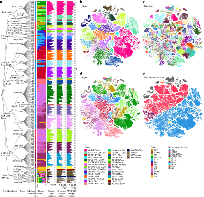
- The final taxonomy contains 34 classes, 338 subclasses, 1,201 supertypes and 5,322 clusters; neuronal types account for 29 classes (85%), 315 subclasses (93%), 1,156 supertypes (96%) and 5,205 clusters (98%), while non-neuronal types form 5 classes, 23 subclasses, 45 supertypes and 117 clusters.
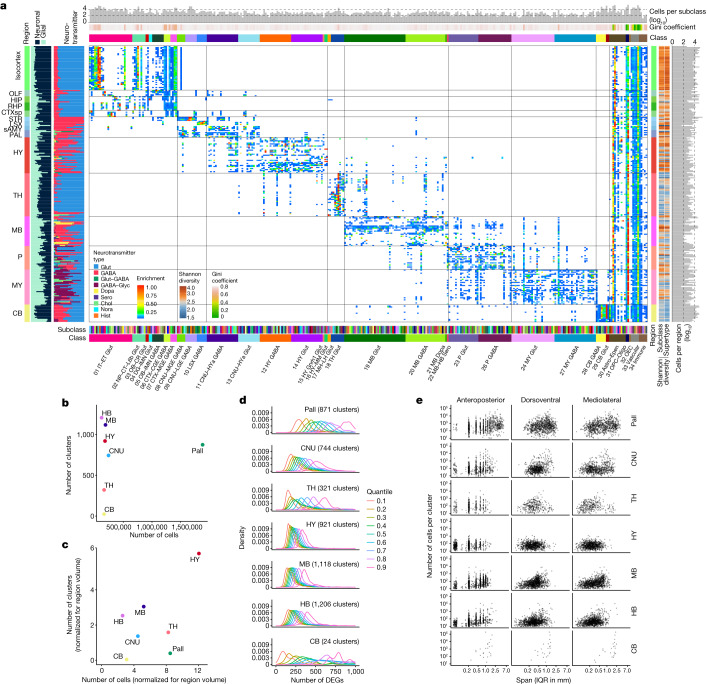
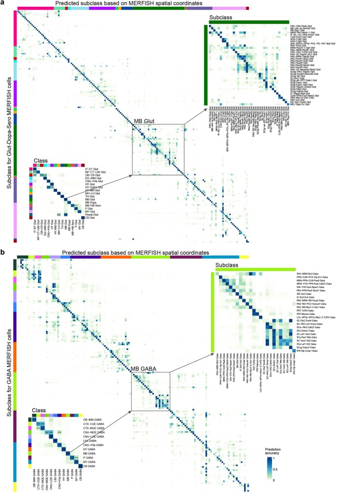
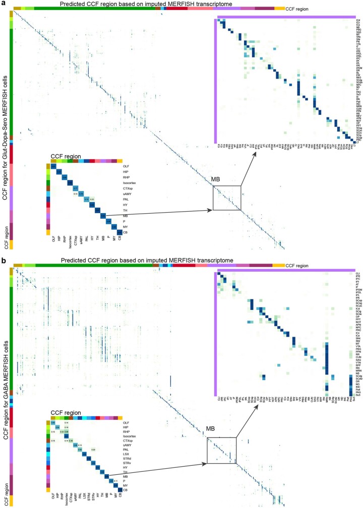
- Neuronal subclasses are spatially restricted, with high inequality in spatial distribution by Gini coefficient and Shannon diversity; transcriptomically similar cell types are spatially closer, and mutual prediction between transcriptomic identity and CCFv3 location is high, with confusions mostly among closely related subclasses or neighbouring regions.
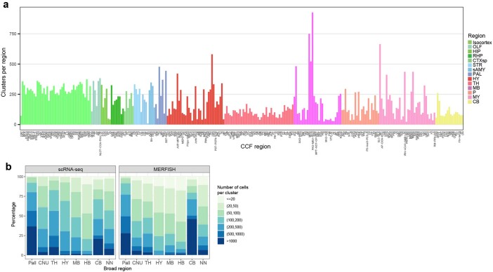
- The brain shows a dorsal–ventral dichotomy: dorsal regions contain fewer yet highly divergent neuronal types, whereas ventral regions contain more numerous, more closely related types; hypothalamus, midbrain and hindbrain have the largest numbers of clusters and smaller spatial spans, while pallium, CNU, thalamus and cerebellum have fewer clusters after volume normalization.
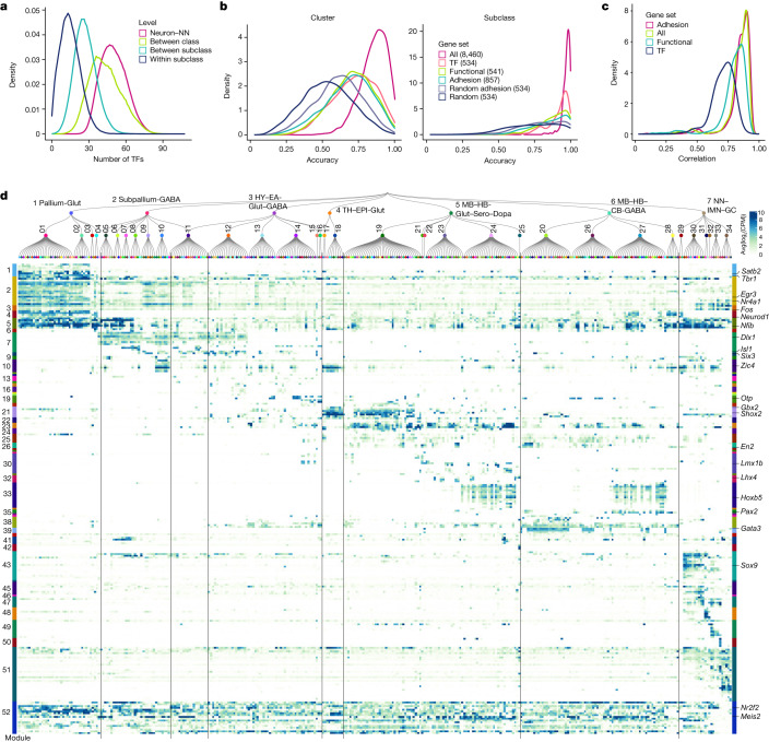
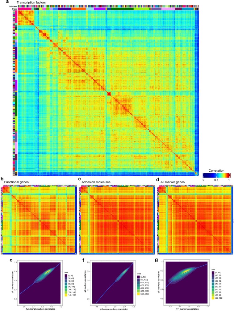
- The study identifies 62 glutamate–GABA dual-transmitter clusters, widespread modulatory neurotransmitter co-release, neuropeptide expression in about 79% of clusters, and 52 transcription factor co-expression modules; transcription factor-based subclass recall is 0.94 versus 0.98 with all DEGs, 0.90 with functional genes, 0.88 with adhesion genes and 0.75 with random DEGs.
Methods
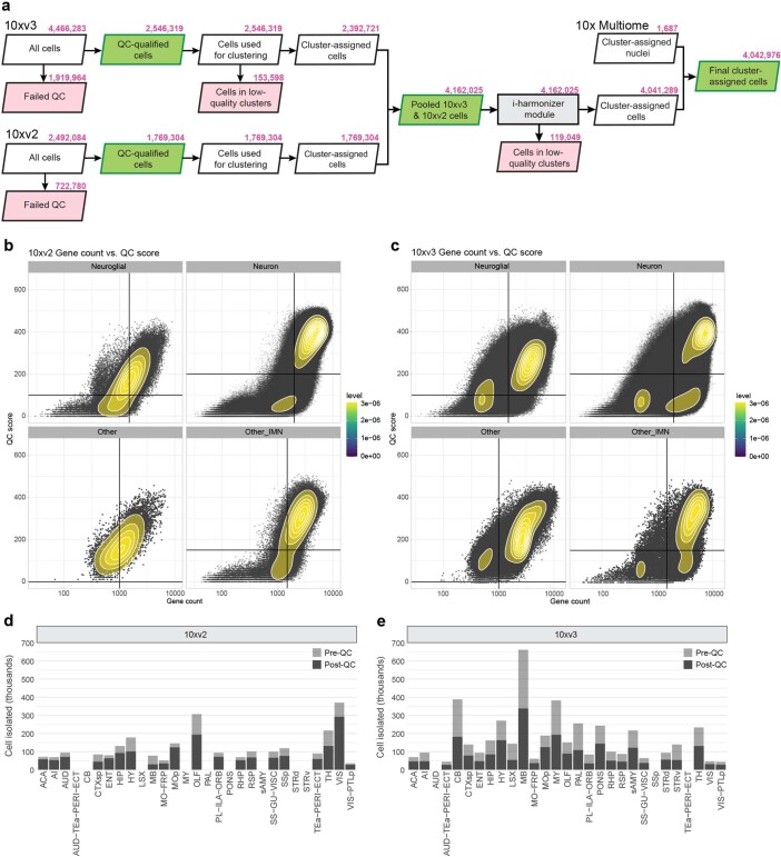
- Generated 781 scRNA-seq libraries from CCFv3-guided microdissections, yielding around 7.0 million single-cell transcriptomes; stringent QC retained around 4.0 million high-quality cells, with 10xv2 and 10xv3 datasets jointly clustered and supplemented by 1,687 10xMulti snRNA-seq nuclei across 33 clusters.
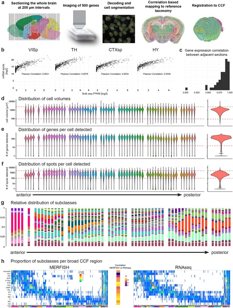
- Used MERFISH with two gene panels (1,147 genes and 500 genes); the AIBS MERFISH dataset comprised 59 serial full coronal sections at 200-µm intervals, around 4.3 million segmented and QC-passed cells, registered to Allen CCFv3 and hierarchically mapped to the scRNA-seq taxonomy.
- Main analyses included iterative clustering, 8,460 differentially expressed marker genes, fivefold cross-validation, UMAP and constellation plots, Gini coefficient and Shannon diversity, mutual prediction between transcriptome and spatial location, and WGCNA for transcription factor modules.
Limitations
- Stated: dissociation of adult brain tissue produced many low-quality cells, damaged cells and mixed debris; stringent QC disqualified a high proportion of cells and likely selectively depleted large neurons such as Purkinje cells and large midbrain/hindbrain motor neurons, so midbrain and hindbrain cell types may not be fully represented or resolved.
- Stated: the complex relationships among cell types cannot be fully captured by a one-dimensional hierarchy or two-dimensional UMAPs; not every cluster may represent a true cell type, and the categorization may need revision with better methods or more experimental evidence, especially developmental data.
- Evident: spatial quantification used only 51/59 MERFISH sections within CCFv3 boundaries and 3,062,367 cells after filtering; 7 small subregions were completely missed, and the authors note that CCFv3 registration inaccuracies may contribute to confusion among neighbouring regions.
Model-written summary. Check it against the paper before relying on it.
Integrity signals
Registry
Cites
Statistics
Figures
Verification
Claims the paper makes
182 Own result · 45 Own interpretation · 38 Own method · 31 No basis given · 28 Partly supported · 19 Supported · 5 No full text of the sources · 3 Supported so far · 3 Not checked yet · 1 Mixed support · 1 Sources not found · accuracy not yet measured
Every source the paper cites for this claim was checked and supports it.
In the paper
“The 10xv3 and 10xv2 cells were first clustered separately and then integrated with methods we developed previously23, resulting in an initial joint transcriptomic cell-type taxonomy with 5,283 clusters (Extended Data Fig. 1a).”
§ A high-resolution transcriptomic and spatial atlas of cell types in the whole mouse brain > Creation of the mouse brain cell-type atlas
What the sources say
- Supportedcites [23] Yao, Z. et al. A taxonomy of transcriptomic cell types across the isocortex and hippocampal formation. Cell 184, 3222–3241.e3226 (2021). source
The citation is attached to the previously developed methods, rather than to the citing study’s 5,283-cluster result. In STAR METHODS (METHOD DETAILS; page unavailable), the source describes independent clustering followed by an integrative clustering method for a joint taxonomy. Its own datasets were 10xv2 and SSv4, so it supports the cited method, not the citing study’s specific datasets or cluster count. (LLM, conf=0.90)
plaindirect- Asserted: passes — The authors put it forward as true.
- Checkable: passes — It can be checked against evidence.
- Load-bearing: passes — The paper’s conclusions depend on it.
- Based: passes — The paper gives a reason why it holds.
- Supported
The cited sources support only part of this claim — read each source’s verdict below.
In the paper
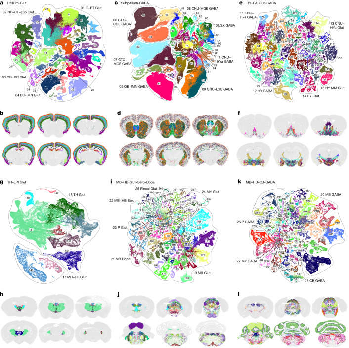
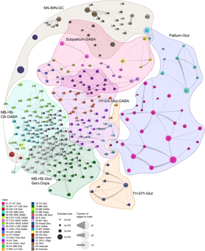
“On the basis of the molecular signature and regional specificity of each subclass, the Subpallium-GABA neighbourhood (subclasses 39–90, total 1,051 clusters) was divided into 7 classes that are likely related to their distinct developmental origins29,30”
§ A high-resolution transcriptomic and spatial atlas of cell types in the whole mouse brain > Neuronal cell types across the mouse brain
What the sources say
- Supportedcites [29] Flames, N. et al. Delineation of multiple subpallial progenitor domains by the combinatorial expression of transcriptional codes. J. Neurosci. 27, 9682–9695 (2007). source
The source supports the developmental-origin rationale: its Introduction describes molecularly distinct subpallial progenitor domains, and its Discussion links different progenitor pools to distinct interneuron populations. The seven-class division and cluster count describe the citing authors’ own classification, not a result attributed to this source. (LLM, conf=0.85)
- Partly supportedcites [30] Turrero Garcia, M. & Harwell, C. C. Radial glia in the ventral telencephalon. FEBS Lett. 591, 3942–3959 (2017). sourceExperimental — accuracy not yet measured
The Introduction says subpallial cell diversity varies with germinal zone and developmental timing, supporting the general link between cell types and developmental origins. The source does not report a Subpallium-GABA neighbourhood, subclasses 39–90, 1,051 clusters, or a division into seven classes. The indexed passages have section labels but no page numbers. (LLM, conf=0.86)
hedgedcorrelational- Asserted: passes — The authors put it forward as true.
- Checkable: passes — It can be checked against evidence.
- Load-bearing: passes — The paper’s conclusions depend on it.
- Based: passes — The paper gives a reason why it holds.
- Supported
The cited sources support only part of this claim — read each source’s verdict below.
In the paper
“We also observed that the NP–CT–L6b-like (NP, near-projecting; CT, corticothalamic; L6b, layer 6b) subclasses emerge as a group highly distinct from the IT–ET-like (IT, intratelencephalic; ET, extratelencephalic) subclasses13,23,26,27, forming two distinct classes, IT–ET Glut and NP–CT–L6b Glut.”
§ A high-resolution transcriptomic and spatial atlas of cell types in the whole mouse brain > Neuronal cell types across the mouse brain
What the sources say
- Partly supportedcites [13] Brain Initiative Cell Census Network. A multimodal cell census and atlas of the mammalian primary motor cortex. Nature 598, 86–102 (2021). sourceExperimental — accuracy not yet measured
The Methods section on L5 ET nomenclature describes a hierarchical taxonomy with distinct IT, L5 ET, L6 CT, NP and L6b glutamatergic subclasses. It does not report that these subclasses form the two named classes, IT–ET Glut and NP–CT–L6b Glut; that grouping is presented as the citing authors’ observation. (LLM, conf=0.84)
- Supportedcites [23] Yao, Z. et al. A taxonomy of transcriptomic cell types across the isocortex and hippocampal formation. Cell 184, 3222–3241.e3226 (2021). source
The Results section on glutamatergic cell type taxonomy places IT neurons, PT (extratelencephalic) neurons, and NP/CT/L6b neurons in separate neighborhoods, supporting the distinction for which this paper is cited. The labels “IT–ET Glut” and “NP–CT–L6b Glut” describe the citing authors’ own two-class observation, not a classification attributed to Yao et al.; page numbers are unavailable in our copy. (LLM, conf=0.86)
- Partly supportedcites [26] Tasic, B. et al. Shared and distinct transcriptomic cell types across neocortical areas. Nature 563, 72–78 (2018). sourceExperimental — accuracy not yet measured
In “Glutamatergic taxonomy by scRNA-seq and projections” (page unavailable), the paper identifies IT, near-projecting and CT as glutamatergic subclasses and describes L6b types. It does not report that NP–CT–L6b and IT–ET form two distinct classes; “Overall cell type taxonomy” instead uses “glutamatergic” as the class and “L6b” as a subclass. (LLM, conf=0.86)
- Supportedcites [27] Yao, Z. et al. A transcriptomic and epigenomic cell atlas of the mouse primary motor cortex. Nature 598, 103–110 (2021). source
The citation is attached to the subclass terminology, while “we also observed” and the proposed two-class grouping describe the citing authors’ own result. The source’s ‘Multimodal molecular census of mouse MOp’ defines NP, CT, L6b, IT and ET as neuronal categories; its Methods (‘Multimodality integration’) also distinguishes excitatory IT from non-IT neurons. The source is therefore appropriate for the cited terminology, without needing to establish the citing authors’ two-class result. (LLM, conf=0.86)
plaincorrelational- Asserted: passes — The authors put it forward as true.
- Checkable: passes — It can be checked against evidence.
- Load-bearing: passes — The paper’s conclusions depend on it.
- Based: passes — The paper gives a reason why it holds.
- Partly supported
Every source the paper cites for this claim was checked and supports it.
In the paper
“We found that the parallel relationships of the different subclasses of glutamatergic neurons between isocortex and HPF that we had reported previously23 extend to other pallium structures—that is, OLF and CTXsp.”
§ A high-resolution transcriptomic and spatial atlas of cell types in the whole mouse brain > Neuronal cell types across the mouse brain
What the sources say
- Supportedcites [23] Yao, Z. et al. A taxonomy of transcriptomic cell types across the isocortex and hippocampal formation. Cell 184, 3222–3241.e3226 (2021). source
The cited paper’s Discussion reports parallel sets of glutamatergic neuron types in the isocortex and hippocampal formation, and its Results describe corresponding subclasses. The extension to OLF and CTXsp is presented in the citing sentence as the citing authors’ new finding, not as a finding attributed to this source. (LLM, conf=0.93)
plaincorrelational- Asserted: passes — The authors put it forward as true.
- Checkable: passes — It can be checked against evidence.
- Load-bearing: passes — The paper’s conclusions depend on it.
- Based: passes — The paper gives a reason why it holds.
- Supported
The cited sources support only part of this claim — read each source’s verdict below.
In the paper
“They include four clusters in the isocortex and hippocampus and three clusters in globus pallidus, internal segment (GPi), which probably correspond to previously well-characterized glutamate–GABA co-releasing neuronal types in these regions41,42.”
§ A high-resolution transcriptomic and spatial atlas of cell types in the whole mouse brain > Neurotransmitter and neuropeptide expression
What the sources say
- Partly supportedcites [41] Kim, S., Wallace, M. L., El-Rifai, M., Knudsen, A. R. & Sabatini, B. L. Co-packaging of opposing neurotransmitters in individual synaptic vesicles in the central nervous system. Neuron 110, 1371–1384.e1377 (2022). sourceExperimental — accuracy not yet measured
Split into 2 atoms — 0 confirmed, 2 partially supported, 0 disputed, 0 misattributed, 0 unverifiable. Expand the claim to see per-atom verdicts.
- Partly supportedcites [42] Pelkey, K. A. et al. Paradoxical network excitation by glutamate release from VGluT3+ GABAergic interneurons. eLife 9, e51996 (2020). sourceExperimental — accuracy not yet measured
Split into 2 atoms — 1 confirmed, 1 partially supported, 0 disputed, 0 misattributed, 0 unverifiable. Expand the claim to see per-atom verdicts.
hedgedcorrelational- Asserted: passes — The authors put it forward as true.
- Checkable: passes — It can be checked against evidence.
- Load-bearing: unclear — It is unclear whether the paper’s conclusions depend on it.
- Based: passes — The paper gives a reason why it holds.
- Partly supported
The cited sources support only part of this claim — read each source’s verdict below.
In the paper
“Both RT and ZI neurons may have originated from the prethalamus or the zona limitans intrathalamica (ZLI)34–38.”
§ A high-resolution transcriptomic and spatial atlas of cell types in the whole mouse brain > Neuronal cell types across the mouse brain
What the sources say
- Not checked — no full text of the sourcecites [34] Delaunay, D. et al. Genetic tracing of subpopulation neurons in the prethalamus of mice (Mus musculus). J. Comp. Neurol. 512, 74–83 (2009). source
- Could not verifycites [35] Govek, K. W. et al. Developmental trajectories of thalamic progenitors revealed by single-cell transcriptome profiling and Shh perturbation. Cell Rep. 41, 111768 (2022). sourceExperimental — accuracy not yet measured
The Results section on molecular identities at E18.5 identifies zona incerta (ZI) and reticular complex (RT) cell populations, while the Introduction describes the ZLI as separating the thalamus from the prethalamus. Neither passage, nor searches for RT and ZI origins, says that both populations may originate in the prethalamus or ZLI. Page numbers were not available in our copy. (LLM, conf=0.72)
- Not checked — no full text of the sourcecites [36] Inamura, N., Ono, K., Takebayashi, H., Zalc, B. & Ikenaka, K. Olig2 lineage cells generate GABAergic neurons in the prethalamic nuclei, including the zona incerta, ventral lateral geniculate nucleus and reticular thalamic nucleus. Dev. Neurosci. 33, 118–129 (2011). source
- Partly supportedcites [37] Puelles, L. et al. LacZ-reporter mapping of Dlx5/6 expression and genoarchitectural analysis of the postnatal mouse prethalamus. J. Comp. Neurol. 529, 367–420 (2021). sourceExperimental — accuracy not yet measured
The Results section, “Regional and areal constitution of the prethalamus” (page unavailable), identifies RT and the rostral and caudal ZI as prethalamic derivatives. The Results section, “Adult prethalamic cell populations at P40 and P140” (page unavailable), instead identifies the zona-limitans-derived retroincertal nucleus as distinct from the caudal ZI; it does not establish a zona limitans origin for both RT and ZI neurons. (LLM, conf=0.86)
- Could not verifycites [38] Shimogori, T. et al. A genomic atlas of mouse hypothalamic development. Nat. Neurosci. 13, 767–775 (2010). sourceExperimental — accuracy not yet measured
The Results section on the anterior diencephalon describes markers of prethalamic neuroepithelium, and the section on basal hypothalamic Shh discusses the ZLI. Neither passage addresses whether RT or ZI neurons originate from either region. Searches for reticular nucleus and zona incerta did not locate a passage establishing that origin. (LLM, conf=0.72)
hedgedconditional- Asserted: passes — The authors put it forward as true.
- Checkable: passes — It can be checked against evidence.
- Load-bearing: unclear — It is unclear whether the paper’s conclusions depend on it.
- Based: passes — The paper gives a reason why it holds.
The cited sources support only part of this claim — read each source’s verdict below.
In the paper
“The HY–EA-Glut–GABA neighbourhood (including subclasses 66 and 73–144, total 1,404 clusters) contains a set of closely related neuronal subclasses from the entire hypothalamus32,33, as well as the striatum-like amygdalar nuclei (sAMY) and caudal PAL regions of CNU that are also known as the extended amygdala”
§ A high-resolution transcriptomic and spatial atlas of cell types in the whole mouse brain > Neuronal cell types across the mouse brain
What the sources say
- Not checked — no full text of the sourcecites [32] Saper, C. B. & Lowell, B. B. The hypothalamus. Curr. Biol. 24, R1111–R1116 (2014). source
- Partly supportedcites [33] Steuernagel, L. et al. HypoMap-a unified single-cell gene expression atlas of the murine hypothalamus. Nat. Metab. 4, 1402–1419 (2022). sourceExperimental — accuracy not yet measured
Split into 2 atoms — 1 confirmed, 0 partially supported, 0 disputed, 0 misattributed, 1 unverifiable. Expand the claim to see per-atom verdicts.
plain- Asserted: passes — The authors put it forward as true.
- Checkable: passes — It can be checked against evidence.
- Load-bearing: passes — The paper’s conclusions depend on it.
- Based: passes — The paper gives a reason why it holds.
Every source the paper cites for this claim was checked and supports it.
In the paper
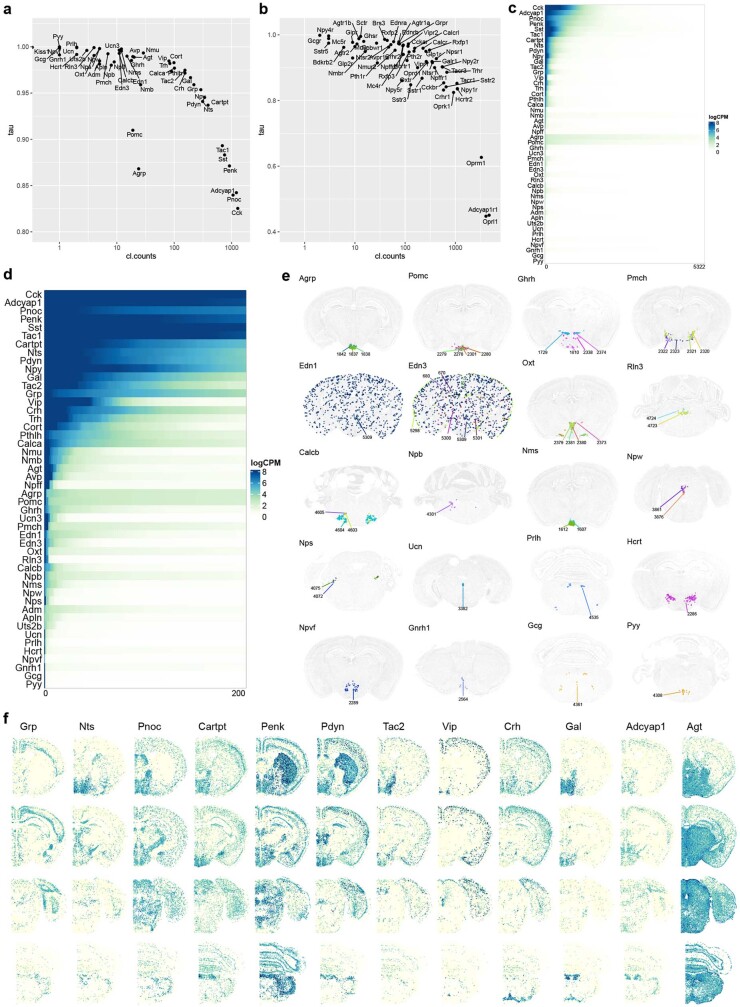
“We measured the cell-type specificity of expression of these genes using the Tau score60 and found a wide range of variation”
§ A high-resolution transcriptomic and spatial atlas of cell types in the whole mouse brain > Neurotransmitter and neuropeptide expression
What the sources say
- Supportedcites [60] Yanai, I. et al. Genome-wide midrange transcription profiles reveal expression level relationships in human tissue specification. Bioinformatics 21, 650–659 (2005). source
The citation identifies the Tau score used as a measure; the citing authors present the wide variation in their genes as their own finding. The paper’s “Tissue specificity index” section defines τ from expression across tissues, and “Distribution of tissue specificities” describes it as a graded measure from 0 to 1. (LLM, conf=0.93)
plain- Asserted: passes — The authors put it forward as true.
- Checkable: passes — It can be checked against evidence.
- Load-bearing: unclear — It is unclear whether the paper’s conclusions depend on it.
- Based: passes — The paper gives a reason why it holds.
- Supported
The cited sources support only part of this claim — read each source’s verdict below.
In the paper
“The HY Gnrh1 Glut class is the hypothalamic Gnrh1 neuronal type developmentally originated from the embryonic olfactory epithelium39.”
§ A high-resolution transcriptomic and spatial atlas of cell types in the whole mouse brain > Neuronal cell types across the mouse brain
What the sources say
- Partly supportedcites [39] Duittoz, A. H. et al. Development of the gonadotropin-releasing hormone system. J. Neuroendocrinol. 34, e13087 (2022). sourceExperimental — accuracy not yet measured
The Introduction and “Olfactory placode and GnRH ontogenesis” section report that GnRH neurons arise in the developing olfactory region and migrate into the forebrain. The paper places their origin in the olfactory placode, likely near the vomeronasal organ primordium, rather than specifically in the olfactory epithelium. It does not identify an “HY Gnrh1 Glut” class or establish that class’s developmental origin; page numbers were not available in our copy. (LLM, conf=0.86)
plaindirect- Asserted: passes — The authors put it forward as true.
- Checkable: passes — It can be checked against evidence.
- Load-bearing: unclear — It is unclear whether the paper’s conclusions depend on it.
- Based: passes — The paper gives a reason why it holds.
- Partly supported
The cited sources support only part of this claim — read each source’s verdict below.
In the paper
“Of all the non-neuronal cell types, the Astro–Epen class exhibits the most diverse spatial patterns68,69.”
§ A high-resolution transcriptomic and spatial atlas of cell types in the whole mouse brain > Non-neuronal and immature neuronal cell types
What the sources say
- Partly supportedcites [68] Endo, F. et al. Molecular basis of astrocyte diversity and morphology across the CNS in health and disease. Science 378, eadc9020 (2022). sourceExperimental — accuracy not yet measured
The Results section, “Region-specific astrocyte genes and pathways” (page unavailable), documents differences among astrocytes across CNS regions. It does not identify an Astro–Epen class or compare its spatial patterns with those of all other non-neuronal cell types, so the claim that it is the most diverse is unsupported. (LLM, conf=0.84)
- Partly supportedcites [69] John Lin, C. C. et al. Identification of diverse astrocyte populations and their malignant analogs. Nat. Neurosci. 20, 396–405 (2017). sourceExperimental — accuracy not yet measured
The Results (page unavailable) describe astrocyte subpopulations across several brain regions and differing locations within the cortex, supporting spatial diversity among astrocytes. The paper does not identify an “Astro–Epen” class or compare its spatial patterns with those of all other non-neuronal cell types, so it does not support the superlative claim. (LLM, conf=0.82)
plain- Asserted: passes — The authors put it forward as true.
- Checkable: passes — It can be checked against evidence.
- Load-bearing: unclear — It is unclear whether the paper’s conclusions depend on it.
- Based: passes — The paper gives a reason why it holds.
- Partly supported
- It may state two separate claims as one. 140
- Probably not a substantial claim. 70
- The quote only partly states this claim. 3
Some cited sources support this claim and some don’t — read each source’s verdict below.
In the paper
“Recent benchmark studies indicate that for simpler integration problems with relatively low biological complexity and relatively small batch effects in scRNA-Seq datasets, linear methods outperform nonlinear, more complex methods136,137, while for complicated integration tasks with large biological complexity and bigger batch effects, nonlinear methods such as scVI/scanVI outperform others138.”
§ A high-resolution transcriptomic and spatial atlas of cell types in the whole mouse brain > Methods > scRNA-seq
What the sources say
- Partly supportedcites [136] Chen, W. et al. A multicenter study benchmarking single-cell RNA sequencing technologies using reference samples. Nat. Biotechnol. 39, 1103–1114 (2021). sourceExperimental — accuracy not yet measured
Split into 2 atoms — 0 confirmed, 1 partially supported, 0 disputed, 0 misattributed, 1 unverifiable. Expand the claim to see per-atom verdicts.
- Disputedcites [137] Tran, H. T. N. et al. A benchmark of batch-effect correction methods for single-cell RNA sequencing data. Genome Biol. 21, 12 (2020). sourceExperimental — accuracy not yet measured
Split into 2 atoms — 0 confirmed, 1 partially supported, 1 disputed, 0 misattributed, 0 unverifiable. Expand the claim to see per-atom verdicts.
Checked by a reasoning model — may be wrong.
- Supportedcites [138] Luecken, M. D. et al. Benchmarking atlas-level data integration in single-cell genomics. Nat. Methods 19, 41–50 (2022). source
Split into 2 atoms — 2 confirmed, 0 partially supported, 0 disputed, 0 misattributed, 0 unverifiable. Expand the claim to see per-atom verdicts.
hedgeddirect- Asserted: passes — The authors put it forward as true.
- Checkable: passes — It can be checked against evidence.
- Load-bearing: passes — The paper’s conclusions depend on it.
- Based: passes — The paper gives a reason why it holds.
It may state two separate claims as one.
- Partly supported
The sources with a verdict support this claim; the rest weren’t checked yet, have no full text we could read, or their verdicts aren’t rated yet.
In the paper
“Single-cell transcriptomics by single-cell RNA sequencing (scRNA-seq) or single-nucleus RNA sequencing (snRNA-seq) provides unprecedented profiling depth and scalability, enabling comprehensive quantitative analysis and classification of cell types at scale2,3,7–9.”
§ A high-resolution transcriptomic and spatial atlas of cell types in the whole mouse brain > Main
What the sources say
- Supportedcites [2] Zeng, H. What is a cell type and how to define it? Cell 185, 2739–2755 (2022). source
The “Approaches to characterize cell types” section says scRNA-seq and snRNA-seq profile thousands of genes per cell, scale to hundreds of thousands or millions of cells, and are used to generate cell-type taxonomies and atlases. This supports the claim’s profiling, scalability, and classification points. (LLM, conf=0.94)
- Not checked — no full text of the sourcecites [3] Zeng, H. & Sanes, J. R. Neuronal cell-type classification: challenges, opportunities and the path forward. Nat. Rev. Neurosci. 18, 530–546 (2017). source
- Not checked — no full text of the sourcecites [7] Poulin, J. F., Tasic, B., Hjerling-Leffler, J., Trimarchi, J. M. & Awatramani, R. Disentangling neural cell diversity using single-cell transcriptomics. Nat. Neurosci. 19, 1131–1141 (2016). source
- Supportedcites [8] Regev, A. et al. The Human Cell Atlas. eLife 6, e27041 (2017). source
The Introduction says massively parallel scRNA-seq assays can profile tens or hundreds of thousands of cells with increasing accuracy and sensitivity, and describes protocols using isolated nuclei. “Taxonomy: cell types” reports that clustering single-cell expression profiles distinguishes cell types and supports prospects for comprehensive cell-type discovery. The paper therefore supports the cited sentence’s broad claim about scalable profiling and classification. (LLM, conf=0.88)
- Not checked — no full text of the sourcecites [9] Shapiro, E., Biezuner, T. & Linnarsson, S. Single-cell sequencing-based technologies will revolutionize whole-organism science. Nat. Rev. Genet. 14, 618–630 (2013). source
plaindirect- Asserted: passes — The authors put it forward as true.
- Checkable: passes — It can be checked against evidence.
- Load-bearing: passes — The paper’s conclusions depend on it.
- Based: passes — The paper gives a reason why it holds.
Probably not a substantial claim.
- Supported
Every source the paper cites for this claim was checked and supports it.
In the paper
“Transcriptomically defined cell types have been shown to exhibit concordant morphological and physiological properties10,11.”
§ A high-resolution transcriptomic and spatial atlas of cell types in the whole mouse brain > Main
What the sources say
- Supportedcites [10] Gouwens, N. W. et al. Integrated morphoelectric and transcriptomic classification of cortical GABAergic cells. Cell 183, 935–953.e919 (2020). source
The Results section on integrated classification states that, in many cases, cells assigned to a transcriptomic type had consistent electrophysiological and morphological features. It also notes exceptions and says one-to-one correspondence was rare; the citing sentence does not claim that concordance holds for every type. (LLM, conf=0.92)
- Supportedcites [11] Scala, F. et al. Phenotypic variation of transcriptomic cell types in mouse motor cortex. Nature 598, 144–150 (2021). source
The Abstract reports distinct morpho-electric phenotypes across broad transcriptomic families and correlated transcriptomic and morpho-electrical variation within families. The Continuous phenotypic variation section likewise reports that neighbouring transcriptomic types showed similar morphological and electrophysiological properties. (LLM, conf=0.90)
plaincorrelational- Asserted: passes — The authors put it forward as true.
- Checkable: passes — It can be checked against evidence.
- Load-bearing: fails — The paper’s conclusions may not depend on it.
- Based: passes — The paper gives a reason why it holds.
Probably not a substantial claim. The paper’s conclusions may not depend on it.
- Supported
Every source the paper cites for this claim was checked and supports it.
In the paper
“In addition, we uncovered relatedness between the Cajal–Retzius (CR) cells mostly found in HPF (subclass 036 HPF CR Glut) and the olfactory bulb (OB) glutamatergic subclass, 035 OB Eomes Ms4a15 Glut, which are likely mitral and tufted cells28, and grouped them into the OB–CR Glut class (Extended Data Fig. 6).”
§ A high-resolution transcriptomic and spatial atlas of cell types in the whole mouse brain > Neuronal cell types across the mouse brain
What the sources say
- Supportedcites [28] Tufo, C. et al. Development of the mammalian main olfactory bulb. Development 149, dev200210 (2022). source
Split into 2 atoms — 2 confirmed, 0 partially supported, 0 disputed, 0 misattributed, 0 unverifiable. Expand the claim to see per-atom verdicts.
hedgedcorrelational- Asserted: passes — The authors put it forward as true.
- Checkable: passes — It can be checked against evidence.
- Load-bearing: unclear — It is unclear whether the paper’s conclusions depend on it.
- Based: passes — The paper gives a reason why it holds.
It may state two separate claims as one.
- Supported
The cited sources support only part of this claim — read each source’s verdict below.
In the paper
“Glutamatergic subclass 168 SPA–SPFm–SPFp–POL–PIL–PoT Sp9 Glut and GABAergic subclass 203 LGv-SPFp-SPFm Nkx2-2 Tcf7l2 Gaba belong to MB Glut and MB GABA classes, respectively, but they are both located in various posterior thalamic nuclei, suggesting potential migration of these neurons from midbrain pretectal area to thalamus40”
§ A high-resolution transcriptomic and spatial atlas of cell types in the whole mouse brain > Neuronal cell types across the mouse brain
What the sources say
- Partly supportedcites [40] Jager, P. et al. Dual midbrain and forebrain origins of thalamic inhibitory interneurons. eLife 10, e59272 (2021). sourceExperimental — accuracy not yet measured
Split into 2 atoms — 0 confirmed, 1 partially supported, 0 disputed, 0 misattributed, 1 unverifiable. Expand the claim to see per-atom verdicts.
hedgedconditional- Asserted: passes — The authors put it forward as true.
- Checkable: passes — It can be checked against evidence.
- Load-bearing: unclear — It is unclear whether the paper’s conclusions depend on it.
- Based: passes — The paper gives a reason why it holds.
It may state two separate claims as one.
- Partly supported
The cited sources support only part of this claim — read each source’s verdict below.
In the paper
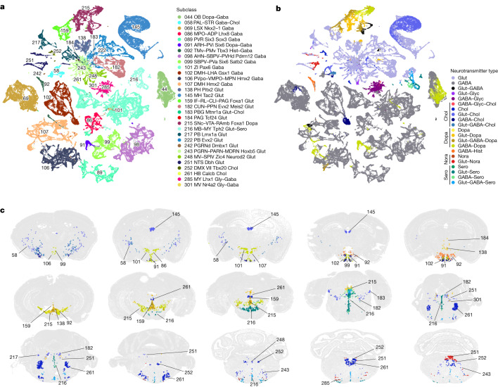
“Cholinergic neurons43,44 are found mainly in subclass 58 in the ventral PAL (11 clusters), but also include 2 clusters in LSX, 8 clusters in MH, 3 clusters in PPN, 5 clusters in dorsal motor nucleus of the vagus nerve (DMX) and nucleus of the solitary tract (NTS), and approximately 13 clusters scattered in other medulla nuclei.”
§ A high-resolution transcriptomic and spatial atlas of cell types in the whole mouse brain > Neurotransmitter and neuropeptide expression
What the sources say
- Partly supportedcites [43] Ahmed, N. Y., Knowles, R. & Dehorter, N. New insights into cholinergic neuron diversity. Frontiers Mol. Neurosci. 12, 204 (2019). sourceExperimental — accuracy not yet measured
The Introduction reports cholinergic neurons in the basal forebrain, medial habenula, and pedunculopontine nucleus, supporting some of the locations named. It does not give the claimed subclass designation or cluster counts, or establish the stated distribution across LSX, DMX, NTS, and other medulla nuclei. (LLM, conf=0.85)
- Partly supportedcites [44] Allaway, K. C. & Machold, R. Developmental specification of forebrain cholinergic neurons. Dev. Biol. 421, 1–7 (2017). sourceExperimental — accuracy not yet measured
The Introduction (page unavailable) identifies cholinergic neurons in the basal forebrain and striatum, supporting the broad point that they occur in forebrain regions. Neither it nor the other retrieved passages gives subclass 58, the listed cluster counts, or the claimed distribution across LSX, MH, PPN, DMX, NTS, and other medulla nuclei. (LLM, conf=0.82)
plain- Asserted: passes — The authors put it forward as true.
- Checkable: passes — It can be checked against evidence.
- Load-bearing: unclear — It is unclear whether the paper’s conclusions depend on it.
- Based: passes — The paper gives a reason why it holds.
It may state two separate claims as one.
- Partly supported
Every source the paper cites for this claim was checked and supports it.
In the paper
“Neuropeptides are also major agents for intercellular communications in the brain58,59.”
§ A high-resolution transcriptomic and spatial atlas of cell types in the whole mouse brain > Neurotransmitter and neuropeptide expression
What the sources say
- Supportedcites [58] Smith, S. J., Hawrylycz, M., Rossier, J. & Sumbul, U. New light on cortical neuropeptides and synaptic network plasticity. Curr. Opin. Neurobiol. 63, 176–188 (2020). source
The Introduction describes neuropeptides as diffusible cell-cell signaling molecules in the brain and says they remain critical to nervous-system function. This supports the claim that they are major agents of intercellular communication there. (LLM, conf=0.94)
- Supportedcites [59] van den Pol, A. N. Neuropeptide transmission in brain circuits. Neuron 76, 98–115 (2012). source
The Abstract says neuropeptides occur in many mammalian CNS neurons and play key roles in modulating neuronal activity. It also describes their release and action through receptors, supporting the broad characterization of neuropeptides as major agents of communication in the brain. (LLM, conf=0.91)
plaindirect- Asserted: passes — The authors put it forward as true.
- Checkable: passes — It can be checked against evidence.
- Load-bearing: fails — The paper’s conclusions may not depend on it.
- Based: passes — The paper gives a reason why it holds.
Probably not a substantial claim. The paper’s conclusions may not depend on it.
- Supported
Every source the paper cites for this claim was checked and supports it.
In the paper
“Although many of these neurotransmitter co-release patterns had been documented previously55–57”
§ A high-resolution transcriptomic and spatial atlas of cell types in the whole mouse brain > Neurotransmitter and neuropeptide expression
What the sources say
- Supportedcites [55] Granger, A. J., Wallace, M. L. & Sabatini, B. L. Multi-transmitter neurons in the mammalian central nervous system. Curr. Opin. Neurobiol. 45, 85–91 (2017). source
The Abstract says that many mammalian neurons are firmly established to release combinations of neurotransmitters. The Introduction describes previously reported examples and points to earlier reviews, supporting the claim that multiple co-release patterns had been documented before. (LLM, conf=0.91)
- Supportedcites [56] Hnasko, T. S. & Edwards, R. H. Neurotransmitter corelease: mechanism and physiological role. Annu. Rev. Physiol. 74, 225–243 (2012). source
The NEUROTRANSMITTER CO-RELEASE section says that exceptions to single-transmitter release had accumulated and describes several previously demonstrated combinations, including ATP with acetylcholine and GABA with glycine. This supports the broad claim that many co-release patterns had already been documented. (LLM, conf=0.92)
- Supportedcites [57] Wallace, M. L. & Sabatini, B. L. Synaptic and circuit functions of multitransmitter neurons in the mammalian brain. Neuron 111, 2969–2983 (2023). source
The Introduction (page not available in our copy) says recent discoveries of multitransmitter neurons were preceded by a long history of study. The review also describes several established forms of neurotransmitter co-release, supporting the claim that many patterns had been documented previously. (LLM, conf=0.88)
plain- Asserted: passes — The authors put it forward as true.
- Checkable: passes — It can be checked against evidence.
- Load-bearing: fails — The paper’s conclusions may not depend on it.
- Based: passes — The paper gives a reason why it holds.
Probably not a substantial claim. The paper’s conclusions may not depend on it.
- Supported
The cited sources support only part of this claim — read each source’s verdict below.
In the paper
“As the immature OB neurons exit the RMS, they express markers such as Sox11 and S100a687, whereas the mature OB neurons are marked by the expression of Frmd7.”
§ A high-resolution transcriptomic and spatial atlas of cell types in the whole mouse brain > Non-neuronal and immature neuronal cell types
What the sources say
- Partly supportedcites [87] Tepe, B. et al. Single-cell RNA-seq of mouse olfactory bulb reveals cellular heterogeneity and activity-dependent molecular census of adult-born neurons. Cell Rep. 25, 2689–2703 e2683 (2018). sourceExperimental — accuracy not yet measured
The Results section, “Transcriptome-Based Clustering of Neurons Identifies Markers of Neuronal Subtypes” (page unavailable), identifies Sox11-enriched cells in the rostral migratory stream as immature migrating adult-born neurons. It does not establish that they express Sox11 as they exit the stream; searches of our copy for S100a6 and Frmd7 found no support for those proposed markers. (LLM, conf=0.86)
plaincorrelational- Asserted: passes — The authors put it forward as true.
- Checkable: passes — It can be checked against evidence.
- Load-bearing: unclear — It is unclear whether the paper’s conclusions depend on it.
- Based: passes — The paper gives a reason why it holds.
It may state two separate claims as one.
- Partly supported
Every source the paper cites for this claim was checked and supports it.
In the paper
“Tanycytes are specialized ependymal cells that line the third ventricle (V3) and the median eminence (ME) in the hypothalamus76.”
§ A high-resolution transcriptomic and spatial atlas of cell types in the whole mouse brain > Non-neuronal and immature neuronal cell types
What the sources say
- Supportedcites [76] Langlet, F., Mullier, A., Bouret, S. G., Prevot, V. & Dehouck, B. Tanycyte-like cells form a blood-cerebrospinal fluid barrier in the circumventricular organs of the mouse brain. J. Comp. Neurol 521, 3389–3405 (2013). source
The Abstract describes tanycytes as highly specialized ependymal cells that line the third ventricle and are apposed to the median eminence. It locates the median eminence in the hypothalamus, supporting the citing sentence’s anatomical description. (LLM, conf=0.93)
plain- Asserted: passes — The authors put it forward as true.
- Checkable: passes — It can be checked against evidence.
- Load-bearing: fails — The paper’s conclusions may not depend on it.
- Based: passes — The paper gives a reason why it holds.
Probably not a substantial claim. The paper’s conclusions may not depend on it.
- Supported
The sources with a verdict support this claim; the rest weren’t checked yet, have no full text we could read, or their verdicts aren’t rated yet.
In the paper
“many of which were well documented61–66.”
§ A high-resolution transcriptomic and spatial atlas of cell types in the whole mouse brain > Non-neuronal and immature neuronal cell types
What the sources say
- Could not verifycites [61] Li, Q. et al. Developmental heterogeneity of microglia and brain myeloid cells revealed by deep single-cell RNA sequencing. Neuron 101, 207–223.e210 (2019). sourceExperimental — accuracy not yet measured
The Results section on phase-specific gene expression says that a majority of newly identified cell-cycle genes appeared in published datasets, but it does not establish that many of the transcription factors in the citing sentence were well documented. Searches for “transcription factors” and “well characterized transcription factors” found no passage making that point; the page number is unavailable in our copy. (LLM, conf=0.72)
- Supportedcites [62] Lozzi, B., Huang, T. W., Sardar, D., Huang, A. Y. & Deneen, B. Regionally distinct astrocytes display unique transcription factor profiles in the adult brain. Front. Neurosci. 14, 61 (2020). source
The Discussion (page unavailable) describes previously established roles for Nkx2-2, Maz, NFIA, and NFIB, supporting the statement that many of the transcription factors were already documented. The paper distinguishes those earlier findings from their roles in adult astrocytes, which it says had not been studied. (LLM, conf=0.84)
- Supportedcites [63] Marques, S. et al. Transcriptional convergence of oligodendrocyte lineage progenitors during development. Dev. Cell 46, 504–517.e507 (2018). source
The Results section (page unavailable) identifies multiple transcription factors involved in patterning and cell specification and names others with roles in oligodendrocyte differentiation. The Discussion (page unavailable) also describes established functions of specific patterning factors. This supports the broad statement that many of these transcription factors were documented. (LLM, conf=0.82)
- Not checked — no full text of the sourcecites [64] Vanlandewijck, M. et al. A molecular atlas of cell types and zonation in the brain vasculature. Nature 554, 475–480 (2018). source
- Supportedcites [65] Yeh, H. & Ikezu, T. Transcriptional and epigenetic regulation of microglia in health and disease. Trends Mol. Med. 25, 96–111 (2019). source
The section ‘Elucidating critical transcriptional regulators of microglial gene expression’ identifies multiple known microglial transcription factors and summarizes studies of their roles. This supports the paraphrase that many of these factors were well documented. (LLM, conf=0.86)
- Supportedcites [66] Zeisel, A. et al. Molecular architecture of the mouse nervous system. Cell 174, 999–1014.e1022 (2018). source
The Results section, “Drivers of Neuronal and Glial Diversity” (page unavailable), discusses many homeodomain transcription factors and their established roles in nervous-system patterning, then documents expression of specific factors. This supports the broad characterization that many of the transcription factors were well documented. (LLM, conf=0.82)
boosted- Asserted: passes — The authors put it forward as true.
- Checkable: passes — It can be checked against evidence.
- Load-bearing: fails — The paper’s conclusions may not depend on it.
- Based: passes — The paper gives a reason why it holds.
Probably not a substantial claim. The paper’s conclusions may not depend on it.
- Could not verify
Every source the paper cites for this claim was checked and supports it.
In the paper
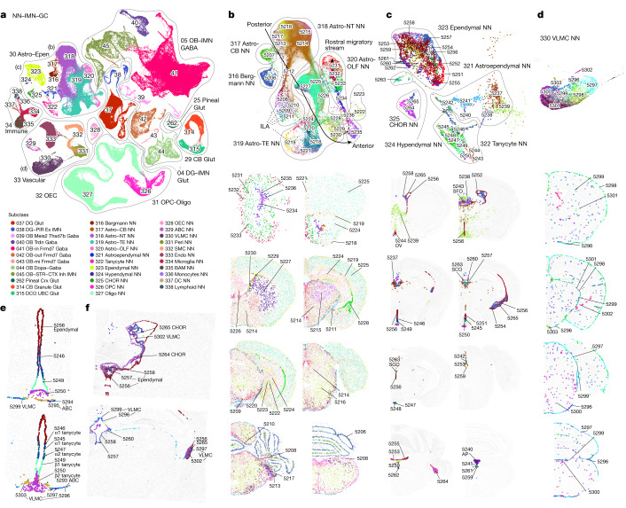
“We also identified tanycyte-like ependymal cell clusters that are specifically located in other CVOs (Fig. 4c): cluster 5243 in the subfornical organ (SFO), 5244 in the vascular organ of the lamina terminalis (OV (also known as OVLT)), 5240 in area postrema (AP), and the hypendymal cell cluster 5263 (marked by Sspo) (Extended Data Fig. 11e) in the subcommissural organ77 (SCO).”
§ A high-resolution transcriptomic and spatial atlas of cell types in the whole mouse brain > Non-neuronal and immature neuronal cell types
What the sources say
- Supportedcites [77] Guerra, M. M. et al. Understanding how the subcommissural organ and other periventricular secretory structures contribute via the cerebrospinal fluid to neurogenesis. Front. Cell. Neurosci. 9, 480 (2015). source
The citation is attached to the subcommissural organ (SCO), not to the citing authors’ identification of numbered clusters. In “The Subcommissural Organ” (page unavailable), the source states that SCO secretory cells form an ependymal and a hypendymal layer, supporting the cited anatomical identification. (LLM, conf=0.90)
plain- Asserted: passes — The authors put it forward as true.
- Checkable: passes — It can be checked against evidence.
- Load-bearing: unclear — It is unclear whether the paper’s conclusions depend on it.
- Based: passes — The paper gives a reason why it holds.
It may state two separate claims as one.
- Supported
Every source the paper cites for this claim was checked and supports it.
In the paper
“Astro-TE cluster 5219 is located at the pia of telencephalon (Fig. 4b) and has high expression of Gfap (Extended Data Fig. 11e), consistent with the definition of interlaminar astrocytes (ILAs)73.”
§ A high-resolution transcriptomic and spatial atlas of cell types in the whole mouse brain > Non-neuronal and immature neuronal cell types
What the sources say
- Supportedcites [73] Falcone, C. et al. Cortical interlaminar astrocytes are generated prenatally, mature postnatally, and express unique markers in human and nonhuman primates. Cereb. Cortex 31, 379–395 (2021). source
The Introduction defines ILAs as GFAP-positive cortical astrocytes and describes pial ILAs as having somata in close contact with the pia. The section on ILA density and morphological complexity likewise identifies ILAs by GFAP expression and a soma contacting the pia. This supports the cited comparison to the ILA definition; the cluster observations are attributed to the citing paper’s figures. (LLM, conf=0.92)
plaincorrelational- Asserted: passes — The authors put it forward as true.
- Checkable: passes — It can be checked against evidence.
- Load-bearing: unclear — It is unclear whether the paper’s conclusions depend on it.
- Based: passes — The paper gives a reason why it holds.
It may state two separate claims as one.
- Supported
The cited sources support only part of this claim — read each source’s verdict below.
In the paper
“The first gives rise to the excitatory DG granule cells, whereas the second produces migrating cells that follow the RMS and in the olfactory bulb differentiate into inhibitory OB granule cells72,84,85.”
§ A high-resolution transcriptomic and spatial atlas of cell types in the whole mouse brain > Non-neuronal and immature neuronal cell types
What the sources say
- Partly supportedcites [72] Lim, D. A. & Alvarez-Buylla, A. The adult ventricular–subventricular zone (V-SVZ) and olfactory bulb (OB) neurogenesis. Cold Spring Harb. Perspect. Biol. 8, a018820 (2016). sourceExperimental — accuracy not yet measured
The Figure 1 caption describes V-SVZ neuroblasts migrating through the RMS into the olfactory bulb and differentiating into granule cells. The section on diverse OB interneurons says most OB granule cells are GABAergic, supporting the inhibitory characterization with that qualifier. The cited paper does not establish the sentence’s separate claim that the dentate gyrus produces excitatory granule cells. (LLM, conf=0.88)
- Partly supportedcites [84] Kempermann, G., Song, H. & Gage, F. H. Neurogenesis in the adult hippocampus. Cold Spring Harb. Perspect. Biol. 7, a018812 (2015). sourceExperimental — accuracy not yet measured
The Abstract (page unavailable) states that adult hippocampal neurogenesis produces excitatory granule cells in the dentate gyrus. The Precursor Cell Phase mentions an SVZ/olfactory-bulb system, but our copy does not say that SVZ-derived cells follow the RMS or differentiate into inhibitory olfactory-bulb granule cells. (LLM, conf=0.86)
- Not checked — no full text of the sourcecites [85] Obernier, K. & Alvarez-Buylla, A. Neural stem cells: origin, heterogeneity and regulation in the adult mammalian brain. Development 146, dev156059 (2019). source
plaindirect- Asserted: passes — The authors put it forward as true.
- Checkable: passes — It can be checked against evidence.
- Load-bearing: unclear — It is unclear whether the paper’s conclusions depend on it.
- Based: passes — The paper gives a reason why it holds.
It may state two separate claims as one.
- Partly supported
The cited sources support only part of this claim — read each source’s verdict below.
In the paper
“Astro-TE clusters 5229 and 5230, located in the lateral ventricle bordering rostral dorsal STR, and clusters belonging to the Astro-OLF subclass (5231–5236) match the path of the RMS70–72 (Extended Data Fig. 12h); the trajectory of these astrocyte clusters on the UMAP matches well with the corresponding spatial gradients”
§ A high-resolution transcriptomic and spatial atlas of cell types in the whole mouse brain > Non-neuronal and immature neuronal cell types
What the sources say
- Partly supportedcites [70] Garcia-Marques, J., De Carlos, J. A., Greer, C. A. & Lopez-Mascaraque, L. Different astroglia permissivity controls the migration of olfactory bulb interneuron precursors. Glia 58, 218–230 (2010). sourceExperimental — accuracy not yet measured
Split into 2 atoms — 0 confirmed, 1 partially supported, 0 disputed, 0 misattributed, 1 unverifiable. Expand the claim to see per-atom verdicts.
- Partly supportedcites [71] Kaneko, N. et al. New neurons clear the path of astrocytic processes for their rapid migration in the adult brain. Neuron 67, 213–223 (2010). sourceExperimental — accuracy not yet measured
Split into 2 atoms — 0 confirmed, 1 partially supported, 0 disputed, 0 misattributed, 1 unverifiable. Expand the claim to see per-atom verdicts.
- Partly supportedcites [72] Lim, D. A. & Alvarez-Buylla, A. The adult ventricular–subventricular zone (V-SVZ) and olfactory bulb (OB) neurogenesis. Cold Spring Harb. Perspect. Biol. 8, a018820 (2016). sourceExperimental — accuracy not yet measured
Split into 2 atoms — 0 confirmed, 1 partially supported, 0 disputed, 0 misattributed, 1 unverifiable. Expand the claim to see per-atom verdicts.
boostedcorrelational- Asserted: passes — The authors put it forward as true.
- Checkable: passes — It can be checked against evidence.
- Load-bearing: passes — The paper’s conclusions depend on it.
- Based: passes — The paper gives a reason why it holds.
It may state two separate claims as one.
- Partly supported
The cited sources support only part of this claim — read each source’s verdict below.
In the paper
“Circumventricular organs (CVOs) are specialized structures located around the third and fourth ventricles that mediate communications between brain, blood and cerebrospinal fluid74,75 (CSF).”
§ A high-resolution transcriptomic and spatial atlas of cell types in the whole mouse brain > Non-neuronal and immature neuronal cell types
What the sources say
- Supportedcites [74] Kiecker, C. The origins of the circumventricular organs. J. Anat. 232, 540–553 (2018). source
The Introduction describes CVOs as specialised neuroepithelial structures grouped around the third and fourth ventricles. It says they provide interfaces between the bloodstream and brain, and between brain tissue and cerebrospinal fluid; the Conclusions likewise describe them as linking all three. (LLM, conf=0.94)
- Partly supportedcites [75] Miyata, S. Glial functions in the blood–brain communication at the circumventricular organs. Front. Neurosci. 16, 991779 (2022). sourceExperimental — accuracy not yet measured
The General introduction says CVOs lie around the brain ventricles and transmit blood-derived information to brain regions. The Abstract and the section on tanycytic transcytosis describe communication between CSF and brain parenchyma. Our copy does not specifically locate CVOs around the third and fourth ventricles, so that more precise part of the claim is not supported. (LLM, conf=0.82)
plaindirect- Asserted: passes — The authors put it forward as true.
- Checkable: passes — It can be checked against evidence.
- Load-bearing: fails — The paper’s conclusions may not depend on it.
- Based: passes — The paper gives a reason why it holds.
Probably not a substantial claim. The paper’s conclusions may not depend on it. It may state two separate claims as one.
- Supported
Every source the paper cites for this claim was checked and supports it.
In the paper
“These observations are consistent with the notion that astrocytes and neurons are derived from common regionally distinct progenitors and share common transcription factors for spatial patterning66,67.”
§ A high-resolution transcriptomic and spatial atlas of cell types in the whole mouse brain > Non-neuronal and immature neuronal cell types
What the sources say
- Supportedcites [66] Zeisel, A. et al. Molecular architecture of the mouse nervous system. Cell 174, 999–1014.e1022 (2018). source
The Results section on neural-crest-derived glia says OPCs are assumed to arise from the same progenitors as astrocytes and neurons. The Results section on neuronal and glial diversity reports the patterning factor Foxg1 in both forebrain neurons and telencephalon-specific astrocytes; the Discussion links their regional patterns to developmental transcription factors. The claim is framed as a notion consistent with these observations, not as a directly demonstrated lineage result. Page numbers were not provided. (LLM, conf=0.88)
- Supportedcites [67] Herrero-Navarro, A. et al. Astrocytes and neurons share region-specific transcriptional signatures that confer regional identity to neuronal reprogramming. Sci. Adv. 7, eabe8978 (2021). source
The Discussion states that neurons and astrocytes have a common developmental origin and share region-identity genes, including transcription factors involved in neuron subtype specification. The Results section on thalamic progenitor clones links their shared region-specific gene expression to common clonal origin and retained positional information. (LLM, conf=0.92)
hedgedcorrelational- Asserted: passes — The authors put it forward as true.
- Checkable: passes — It can be checked against evidence.
- Load-bearing: unclear — It is unclear whether the paper’s conclusions depend on it.
- Based: passes — The paper gives a reason why it holds.
It may state two separate claims as one.
- Supported
The cited sources support only part of this claim — read each source’s verdict below.
In the paper
“Although their loci are not very near to each other, Nfia, Nfib and Nfix regulate cell-type differentiation in many tissues94–96, function as homo- or heterodimers, and bind to largely common targets97.”
§ A high-resolution transcriptomic and spatial atlas of cell types in the whole mouse brain > Transcription factors in defining cell types
What the sources say
- Partly supportedcites [94] Campbell, C. E. et al. The transcription factor Nfix is essential for normal brain development. BMC Dev. Biol. 8, 52 (2008). sourceExperimental — accuracy not yet measured
The Background states that NFI proteins form homo- or heterodimers, and the Discussion says Nfia, Nfib and Nfix have important roles in brain development and that NFI proteins appear to bind the same DNA sequences. But the Discussion explicitly leaves open whether the proteins share target genes, so it does not establish that they bind largely common targets. It also does not establish cell-type differentiation by all three across many tissues. (LLM, conf=0.84)
- Partly supportedcites [95] Holmfeldt, P. et al. Nfix is a novel regulator of murine hematopoietic stem and progenitor cell survival. Blood 122, 2987–2996 (2013). sourceExperimental — accuracy not yet measured
The Introduction (page unavailable) reports roles for Nfix in muscle and neural development and for Nfia in a blood-cell lineage switch; it also describes a lung-development defect in Nfib-deficient mice. This supports a broad developmental role for the family, but does not establish that all three genes regulate cell-type differentiation across many tissues. The separate citation attached to dimerization and common targets is not attributed to this paper. (LLM, conf=0.83)
- Not checked — no full text of the sourcecites [96] Messina, G. et al. Nfix regulates fetal-specific transcription in developing skeletal muscle. Cell 140, 554–566 (2010). source
- Partly supportedcites [97] Fraser, J. et al. Common regulatory targets of NFIA, NFIX and NFIB during postnatal cerebellar development. Cerebellum 19, 89–101 (2020). sourceExperimental — accuracy not yet measured
The Results (page unavailable) show substantial overlap in NFIA, NFIB and NFIX binding sites in postnatal cerebellar cells. The Discussion (page unavailable) says heterodimerisation is known in vitro but its prevalence in vivo is unclear; it does not establish that these proteins function as heterodimers in vivo or address homodimerisation. The earlier claims about locus proximity and differentiation across tissues carry different citations and are not assessed here. (LLM, conf=0.88)
plaindirect- Asserted: passes — The authors put it forward as true.
- Checkable: passes — It can be checked against evidence.
- Load-bearing: fails — The paper’s conclusions may not depend on it.
- Based: passes — The paper gives a reason why it holds.
Probably not a substantial claim. The paper’s conclusions may not depend on it. It may state two separate claims as one.
- Partly supported
The cited sources support only part of this claim — read each source’s verdict below.
In the paper
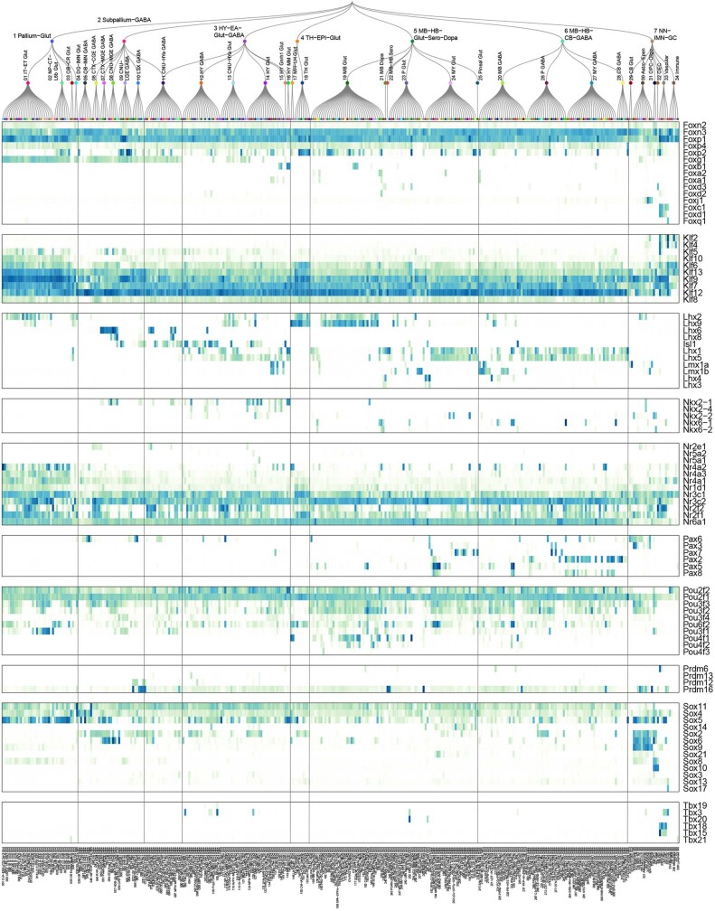
“We examined the expression patterns of several transcription factor families (Extended Data Fig. 13), including forkhead box (Fox), Krüppel-like factor (Klf), LIM homeobox (Lhx), NKX-homeodomain (Nkx), nuclear receptor (Nr), Paired box (Pax), POU domain (Pou), positive regulatory domain (Prdm), SRY-related HMG-box (Sox), and T-box (Tbx), all of which have been shown to have important roles in”
§ A high-resolution transcriptomic and spatial atlas of cell types in the whole mouse brain > Transcription factors in defining cell types
What the sources say
- Partly supportedcites [100] Golson, M. L. & Kaestner, K. H. Fox transcription factors: from development to disease. Development 143, 4558–4570 (2016). sourceExperimental — accuracy not yet measured
Split into 2 atoms — 0 confirmed, 2 partially supported, 0 disputed, 0 misattributed, 0 unverifiable. Expand the claim to see per-atom verdicts.
- Not checked — no full text of the sourcecites [101] Hohenauer, T. & Moore, A. W. The Prdm family: expanding roles in stem cells and development. Development 139, 2267–2282 (2012). source
- Partly supportedcites [102] Malik, V., Zimmer, D. & Jauch, R. Diversity among POU transcription factors in chromatin recognition and cell fate reprogramming. Cell. Mol. Life Sci. 75, 1587–1612 (2018). sourceExperimental — accuracy not yet measured
Split into 2 atoms — 0 confirmed, 2 partially supported, 0 disputed, 0 misattributed, 0 unverifiable. Expand the claim to see per-atom verdicts.
- Partly supportedcites [103] Presnell, J. S., Schnitzler, C. E. & Browne, W. E. KLF/SP transcription factor family evolution: expansion, diversification, and innovation in eukaryotes. Genome Biol. Evol. 7, 2289–2309 (2015). sourceExperimental — accuracy not yet measured
Split into 2 atoms — 0 confirmed, 1 partially supported, 0 disputed, 0 misattributed, 1 unverifiable. Expand the claim to see per-atom verdicts.
- Partly supportedcites [104] Prior, H. M. & Walter, M. A. SOX genes: architects of development. Mol. Med. 2, 405–412 (1996). sourceExperimental — accuracy not yet measured
Split into 2 atoms — 0 confirmed, 2 partially supported, 0 disputed, 0 misattributed, 0 unverifiable. Expand the claim to see per-atom verdicts.
- Partly supportedcites [105] Sever, R. & Glass, C. K. Signaling by nuclear receptors. Cold Spring Harb. Perspect. Biol. 5, a016709 (2013). sourceExperimental — accuracy not yet measured
Split into 2 atoms — 0 confirmed, 1 partially supported, 0 disputed, 0 misattributed, 1 unverifiable. Expand the claim to see per-atom verdicts.
- Partly supportedcites [106] Srivastava, M. et al. Early evolution of the LIM homeobox gene family. BMC Biol. 8, 4 (2010). sourceExperimental — accuracy not yet measured
Split into 2 atoms — 0 confirmed, 2 partially supported, 0 disputed, 0 misattributed, 0 unverifiable. Expand the claim to see per-atom verdicts.
- Not checked — no full text of the sourcecites [107] Stanfel, M. N., Moses, K. A., Schwartz, R. J. & Zimmer, W. E. Regulation of organ development by the NKX-homeodomain factors: an NKX code. Cell. Mol. Biol. 51, OL785–OL799 (2005).
plaincorrelational- Asserted: passes — The authors put it forward as true.
- Checkable: passes — It can be checked against evidence.
- Load-bearing: fails — The paper’s conclusions may not depend on it.
- Based: passes — The paper gives a reason why it holds.
Probably not a substantial claim. The paper’s conclusions may not depend on it. It may state two separate claims as one.
- Partly supported
The cited sources support only part of this claim — read each source’s verdict below.
In the paper
“Isl1 is widely expressed in hypothalamus and CNU, and more highly in GABAergic than glutamatergic cell types115.”
§ A high-resolution transcriptomic and spatial atlas of cell types in the whole mouse brain > Transcription factors in defining cell types
What the sources say
- Partly supportedcites [115] Ehrman, L. A. et al. The LIM homeobox gene Isl1 is required for the correct development of the striatonigral pathway in the mouse. Proc. Natl Acad. Sci. USA 110, E4026–E4035 (2013). sourceExperimental — accuracy not yet measured
The Results (page unavailable) report Isl1 expression in a subpopulation of developing striatal neurons and in adult neurons of the rTh and zona incerta; fate-mapped striatal neurons have characteristics of GABAergic projection neurons. The paper does not establish widespread expression across the hypothalamus and CNU or compare Isl1 expression levels in GABAergic and glutamatergic cell types. (LLM, conf=0.83)
plaincorrelational- Asserted: passes — The authors put it forward as true.
- Checkable: passes — It can be checked against evidence.
- Load-bearing: unclear — It is unclear whether the paper’s conclusions depend on it.
- Based: passes — The paper gives a reason why it holds.
It may state two separate claims as one.
- Partly supported
The cited sources support only part of this claim — read each source’s verdict below.
In the paper
“Gbx2, Shox2 and Tcf7l2 are highly expressed in thalamus glutamatergic neurons91,92, whereas Shox2 and Tcf7l2 are also expressed in midbrain.”
§ A high-resolution transcriptomic and spatial atlas of cell types in the whole mouse brain > Transcription factors in defining cell types
What the sources say
- Partly supportedcites [91] Lee, M. et al. Tcf7l2 plays crucial roles in forebrain development through regulation of thalamic and habenular neuron identity and connectivity. Dev. Biol. 424, 62–76 (2017). sourceExperimental — accuracy not yet measured
Section 2.1 reports high Tcf7l2 expression in thalamic neurons and substantial overlap with Gbx2 in the caudal thalamic mantle zone. Our copy does not establish that these cells are glutamatergic or report Shox2 expression. The midbrain clause follows the citations and is not clearly attributed to this source. (LLM, conf=0.86)
- Partly supportedcites [92] Mallika, C., Guo, Q. & Li, J. Y. Gbx2 is essential for maintaining thalamic neuron identity and repressing habenular characters in the developing thalamus. Dev. Biol. 407, 26–39 (2015). sourceExperimental — accuracy not yet measured
The Introduction (page unavailable) says Gbx2 is expressed in thalamic neuronal precursors and remains expressed in mature thalamic neurons. It does not establish that these are glutamatergic neurons, and the passages retrieved for Shox2 and Tcf7l2 do not establish their thalamic expression. The midbrain clause follows the citations and is not treated as attributed to this paper. (LLM, conf=0.83)
plaincorrelational- Asserted: passes — The authors put it forward as true.
- Checkable: passes — It can be checked against evidence.
- Load-bearing: unclear — It is unclear whether the paper’s conclusions depend on it.
- Based: passes — The paper gives a reason why it holds.
It may state two separate claims as one.
- Partly supported
The cited sources support only part of this claim — read each source’s verdict below.
In the paper
“Similar interactions between homologues have been reported for many other transcription factor families, such as Ebf98 and Irx99.”
§ A high-resolution transcriptomic and spatial atlas of cell types in the whole mouse brain > Transcription factors in defining cell types
What the sources say
- Partly supportedcites [98] Siponen, M. I. et al. Structural determination of functional domains in early B-cell factor (EBF) family of transcription factors reveals similarities to Rel DNA-binding proteins and a novel dimerization motif. J. Biol. Chem. 285, 25875–25879 (2010). sourceExperimental — accuracy not yet measured
The Results (page unavailable) report dimer formation in both EBF1 and EBF3 crystals, supporting interactions between EBF molecules. They do not report an interaction between different EBF homologues, such as EBF1 with EBF3. The separate Irx citation is outside the scope of this verdict. (LLM, conf=0.83)
- Supportedcites [99] Bilioni, A., Craig, G., Hill, C. & McNeill, H. Iroquois transcription factors recognize a unique motif to mediate transcriptional repression in vivo. Proc. Natl Acad. Sci. USA 102, 14671–14676 (2005). source
The Results section reports that Iro/Irx transcription factors form homodimers and heterodimers. The Discussion says EMSA and pull-down assays confirmed these interactions in vitro, supporting the citing sentence’s Irx example; the separate Ebf citation is not being judged here. (LLM, conf=0.93)
plaincorrelational- Asserted: passes — The authors put it forward as true.
- Checkable: passes — It can be checked against evidence.
- Load-bearing: fails — The paper’s conclusions may not depend on it.
- Based: passes — The paper gives a reason why it holds.
Probably not a substantial claim. The paper’s conclusions may not depend on it.
- Partly supported
Every source the paper cites for this claim was checked and supports it.
In the paper
“Consistent with the well-studied roles of Hox genes in regulating anterior–posterior axis in development93, Hoxb2 and Hoxb3 have broader expression than Hoxb4 and Hoxb5, and Hoxb8 has the most restricted expression pattern in posterior lateral medulla, in the order that is consistent with their locations on the chromosome.”
§ A high-resolution transcriptomic and spatial atlas of cell types in the whole mouse brain > Transcription factors in defining cell types
What the sources say
- Supportedcites [93] Philippidou, P. & Dasen, J. S. Hox genes: choreographers in neural development, architects of circuit organization. Neuron 80, 12–34 (2013). source
Split into 2 atoms — 2 confirmed, 0 partially supported, 0 disputed, 0 misattributed, 0 unverifiable. Expand the claim to see per-atom verdicts.
boostedcorrelational- Asserted: passes — The authors put it forward as true.
- Checkable: passes — It can be checked against evidence.
- Load-bearing: unclear — It is unclear whether the paper’s conclusions depend on it.
- Based: passes — The paper gives a reason why it holds.
It may state two separate claims as one.
- Supported
The cited sources support only part of this claim — read each source’s verdict below.
In the paper
“Lhx2 and Lhx9 are co-expressed in thalamus and midbrain glutamatergic types, but Lhx2 is also specifically expressed in the pallium IT–ET types108,109.”
§ A high-resolution transcriptomic and spatial atlas of cell types in the whole mouse brain > Transcription factors in defining cell types
What the sources say
- Partly supportedcites [108] Matho, K. S. et al. Genetic dissection of the glutamatergic neuron system in cerebral cortex. Nature 598, 182–187 (2021). sourceExperimental — accuracy not yet measured
The Fate-mapping PyN progenitors > RGs section (page unavailable) reports Lhx2-positive progenitors in the dorsal pallium that give rise to IT and ET neurons. It does not establish that Lhx2 is specifically expressed in the IT–ET neuron types themselves, and a search for Lhx9 found no passage about its co-expression with Lhx2 in thalamic or midbrain glutamatergic types. (LLM, conf=0.87)
- Partly supportedcites [109] Peukert, D., Weber, S., Lumsden, A. & Scholpp, S. Lhx2 and Lhx9 determine neuronal differentiation and compartition in the caudal forebrain by regulating Wnt signaling. PLoS Biol. 9, e1001218 (2011). sourceExperimental — accuracy not yet measured
The Results section, “Fine Mapping of the Temporal and Spatial Expression of Lhx2 and Lhx9 in the Caudal Diencephalon” (page unavailable), reports Lhx2/Lhx9 co-expression in the zebrafish thalamus and places Lhx9 expression in a glutamatergic thalamic domain. It does not establish co-expression in midbrain glutamatergic types or specific Lhx2 expression in pallium IT–ET types; the Discussion mentions the pallium without identifying those cell types. (LLM, conf=0.88)
plaincorrelational- Asserted: passes — The authors put it forward as true.
- Checkable: passes — It can be checked against evidence.
- Load-bearing: unclear — It is unclear whether the paper’s conclusions depend on it.
- Based: passes — The paper gives a reason why it holds.
It may state two separate claims as one.
- Partly supported
The cited sources support only part of this claim — read each source’s verdict below.
In the paper
“Lmx1a and Lmx1b are co-expressed in hindbrain glutamatergic and midbrain dopaminergic cell types112, and Lmx1b is also specifically expressed in serotonergic types113,114.”
§ A high-resolution transcriptomic and spatial atlas of cell types in the whole mouse brain > Transcription factors in defining cell types
What the sources say
- Partly supportedcites [112] Yan, C. H., Levesque, M., Claxton, S., Johnson, R. L. & Ang, S. L. Lmx1a and Lmx1b function cooperatively to regulate proliferation, specification, and differentiation of midbrain dopaminergic progenitors. J. Neurosci. 31, 12413–12425 (2011). sourceExperimental — accuracy not yet measured
The Introduction says midbrain dopaminergic progenitors express both Lmx1a and Lmx1b, and the section on postmitotic mDA neurons describes precursors expressing both. Our copy does not establish their co-expression in hindbrain glutamatergic cell types. The serotonergic clause is attached to citations 113 and 114, not this source. (LLM, conf=0.86)
- Partly supportedcites [113] Cheng, L. et al. Lmx1b, Pet-1, and Nkx2.2 coordinately specify serotonergic neurotransmitter phenotype. J. Neurosci. 23, 9961–9967 (2003). sourceExperimental — accuracy not yet measured
The section “Lmx1b is expressed in developing serotonergic neurons” reports Lmx1b in all 5-HT neurons, supporting the clause attributed to this paper. It also reports Lmx1b-positive neurons that are 5-HT-negative, so the evidence does not support “specifically” if that means exclusive expression in serotonergic cells. The preceding co-expression clause is attached to citation 112, not this source. (LLM, conf=0.86)
- Not checked — no full text of the sourcecites [114] Ding, Y. Q. et al. Lmx1b is essential for the development of serotonergic neurons. Nat. Neurosci. 6, 933–938 (2003). source
plaincorrelational- Asserted: passes — The authors put it forward as true.
- Checkable: passes — It can be checked against evidence.
- Load-bearing: unclear — It is unclear whether the paper’s conclusions depend on it.
- Based: passes — The paper gives a reason why it holds.
It may state two separate claims as one.
- Partly supported
Every source the paper cites for this claim was checked and supports it.
In the paper
“The grouping of Lhx members based on their gene expression patterns exactly matches their phylogeny tree based on their coding sequences106 and aligns with the sub-family definition.”
§ A high-resolution transcriptomic and spatial atlas of cell types in the whole mouse brain > Transcription factors in defining cell types
What the sources say
- Supportedcites [106] Srivastava, M. et al. Early evolution of the LIM homeobox gene family. BMC Biol. 8, 4 (2010). source
The citation is attached to the sequence-based phylogeny, rather than to the citing authors’ comparison with their expression-pattern grouping. The Methods (Phylogenetic analyses and identification of introns; page unavailable) describe aligning Lhx sequences and constructing phylogenetic trees, and the Results (Origin and early diversification; page unavailable) use the tree to assign genes to subfamilies. The source does not itself establish an exact match with expression-pattern groupings. (LLM, conf=0.88)
plaincorrelational- Asserted: passes — The authors put it forward as true.
- Checkable: passes — It can be checked against evidence.
- Load-bearing: unclear — It is unclear whether the paper’s conclusions depend on it.
- Based: passes — The paper gives a reason why it holds.
It may state two separate claims as one.
- Supported
The cited sources support only part of this claim — read each source’s verdict below.
In the paper
“Lhx6 and Lhx8 are co-expressed in some CNU and hypothalamus GABAergic types110,111, but Lhx6 is also specifically expressed in MGE types.”
§ A high-resolution transcriptomic and spatial atlas of cell types in the whole mouse brain > Transcription factors in defining cell types
What the sources say
- Partly supportedcites [110] Flandin, P. et al. Lhx6 and Lhx8 coordinately induce neuronal expression of Shh that controls the generation of interneuron progenitors. Neuron 70, 939–950 (2011). sourceExperimental — accuracy not yet measured
The Results section reports Lhx6 and Lhx8 coexpression in more than 90% of cells in the embryonic MGE subventricular zone (page unavailable). The Discussion links both genes to striatal interneuron development, but our copy does not establish their coexpression in the cited CNU GABAergic types or address hypothalamic GABAergic types. (LLM, conf=0.84)
- Partly supportedcites [111] Fragkouli, A., van Wijk, N. V., Lopes, R., Kessaris, N. & Pachnis, V. LIM homeodomain transcription factor-dependent specification of bipotential MGE progenitors into cholinergic and GABAergic striatal interneurons. Development 136, 3841–3851 (2009). sourceExperimental — accuracy not yet measured
The Results (page unavailable) show Lhx6 in a subset of Lhx7-reporter-positive striatal cells; the Introduction identifies Lhx7 as Lhx8. The Discussion (page unavailable) reports Lhx7-reporter expression in hypothalamic GABAergic neurons, but does not establish that those neurons also express Lhx6. (LLM, conf=0.86)
plaincorrelational- Asserted: passes — The authors put it forward as true.
- Checkable: passes — It can be checked against evidence.
- Load-bearing: unclear — It is unclear whether the paper’s conclusions depend on it.
- Based: passes — The paper gives a reason why it holds.
It may state two separate claims as one.
- Partly supported
The cited sources support only part of this claim — read each source’s verdict below.
In the paper
“Clustering for both 10xv2 and 10xv3 datasets was performed independently using the in-house developed R package scrattch.bigcat (v0.0.5, available via github https://github.com/AllenInstitute/scrattch.bigcat), which is a scaled-up version of R package scrattch.hicat23,26 to deal with the increased size of datasets.”
§ A high-resolution transcriptomic and spatial atlas of cell types in the whole mouse brain > Methods > scRNA-seq
What the sources say
- Partly supportedcites [23] Yao, Z. et al. A taxonomy of transcriptomic cell types across the isocortex and hippocampal formation. Cell 184, 3222–3241.e3226 (2021). sourceExperimental — accuracy not yet measured
In STAR METHODS > METHOD DETAILS (page not supplied), the paper says it adapted scrattch.hicat into scrattch.bigcat for the large 10xv2 dataset. Its independent-clustering description instead names SSv4 and 10xv2 and says they used scrattch.hicat; it does not support the claim about independently clustering 10xv3 with scrattch.bigcat. (LLM, conf=0.88)
- Supportedcites [26] Tasic, B. et al. Shared and distinct transcriptomic cell types across neocortical areas. Nature 563, 72–78 (2018). source
The citation is attached to scrattch.hicat, identifying the earlier R package rather than supporting the citing paper’s claim about its 10x datasets or scrattch.bigcat. The source’s Methods, under Code availability, identifies scrattch.hicat as its R package for iterative clustering. (LLM, conf=0.92)
plain- Asserted: passes — The authors put it forward as true.
- Checkable: passes — It can be checked against evidence.
- Load-bearing: fails — The paper’s conclusions may not depend on it.
- Based: passes — The paper gives a reason why it holds.
Probably not a substantial claim. The paper’s conclusions may not depend on it.
- Partly supported
Every source the paper cites for this claim was checked and supports it.
In the paper
“Given the significant increase of data size and complexities of the taxonomy, we re-implemented this method that provides essentially identical results, but drastically improves performance and scalability.”
§ A high-resolution transcriptomic and spatial atlas of cell types in the whole mouse brain > Methods > scRNA-seq
What the sources say
- Supportedcites [133] Ritchie, M. E. et al. limma powers differential expression analyses for RNA-sequencing and microarray studies. Nucleic Acids Res. 43, e47 (2015). source
The Results section (‘Finding differentially expressed genes’; page not provided) identifies limma’s gene-wise linear modelling as a method for assessing differential expression. The citing sentence describes the authors’ own re-implementation and its reported results; it uses this source to identify the method, not to substantiate their performance comparison. (LLM, conf=0.88)
plaindirect- Asserted: passes — The authors put it forward as true.
- Checkable: passes — It can be checked against evidence.
- Load-bearing: unclear — It is unclear whether the paper’s conclusions depend on it.
- Based: passes — The paper gives a reason why it holds.
It may state two separate claims as one.
- Supported
Every source the paper cites for this claim was checked and supports it.
In the paper
“Consistent with the principle of hierarchical cell-type organization identified in previous studies2, here we have defined a hierarchical taxonomy of cell types across the entire mouse brain, with four levels of classification: class, subclass, supertype and cluster (or type).”
§ A high-resolution transcriptomic and spatial atlas of cell types in the whole mouse brain > Discussion
What the sources say
- Supportedcites [2] Zeng, H. What is a cell type and how to define it? Cell 185, 2739–2755 (2022). source
Split into 2 atoms — 2 confirmed, 0 partially supported, 0 disputed, 0 misattributed, 0 unverifiable. Expand the claim to see per-atom verdicts.
plain- Asserted: passes — The authors put it forward as true.
- Checkable: passes — It can be checked against evidence.
- Load-bearing: passes — The paper’s conclusions depend on it.
- Based: passes — The paper gives a reason why it holds.
Probably not a substantial claim.
- Supported
Every source the paper cites for this claim was checked and supports it.
In the paper
“Doublets were identified using a modified version of the DoubletFinder algorithm132 (available in scrattch.hicat, https://github.com/AllenInstitute/scrattch.hicat, v1.0.9) and removed when doublet score >0.3.”
§ A high-resolution transcriptomic and spatial atlas of cell types in the whole mouse brain > Methods > scRNA-seq
What the sources say
- Supportedcites [132] McGinnis, C. S., Murrow, L. M. & Gartner, Z. J. DoubletFinder: doublet detection in single-cell RNA sequencing data using artificial nearest neighbors. Cell Syst. 8, 329–337.e324 (2019). source
The Results section (‘Overview of DoubletFinder’) describes the DoubletFinder algorithm for predicting doublets. The citation is attached to the algorithm’s name; the modified implementation and >0.3 removal threshold describe the citing authors’ procedure, not a threshold attributed to this source. (LLM, conf=0.92)
plaindirect- Asserted: passes — The authors put it forward as true.
- Checkable: passes — It can be checked against evidence.
- Load-bearing: passes — The paper’s conclusions depend on it.
- Based: passes — The paper gives a reason why it holds.
Probably not a substantial claim. It may state two separate claims as one.
- Supported
Every source the paper cites for this claim was checked and supports it.
In the paper
“Of note, our assignment of neurotransmitter types based on synthesizing enzymes and transporter genes is conservative; there may be even more diversity in neurotransmitter co-release patterns if other unconventional transmitter release routes are considered57,118.”
§ A high-resolution transcriptomic and spatial atlas of cell types in the whole mouse brain > Discussion
What the sources say
- Supportedcites [57] Wallace, M. L. & Sabatini, B. L. Synaptic and circuit functions of multitransmitter neurons in the mammalian brain. Neuron 111, 2969–2983 (2023). source
Split into 2 atoms — 2 confirmed, 0 partially supported, 0 disputed, 0 misattributed, 0 unverifiable. Expand the claim to see per-atom verdicts.
- Supportedcites [118] Melani, R. & Tritsch, N. X. Inhibitory co-transmission from midbrain dopamine neurons relies on presynaptic GABA uptake. Cell Rep. 39, 110716 (2022). source
Split into 2 atoms — 2 confirmed, 0 partially supported, 0 disputed, 0 misattributed, 0 unverifiable. Expand the claim to see per-atom verdicts.
hedgedconditional- Asserted: passes — The authors put it forward as true.
- Checkable: passes — It can be checked against evidence.
- Load-bearing: unclear — It is unclear whether the paper’s conclusions depend on it.
- Based: passes — The paper gives a reason why it holds.
It may state two separate claims as one.
- Supported
The cited sources support only part of this claim — read each source’s verdict below.
In the paper
“It is known that in many midbrain dopamine neurons (in VTA and SNc), Aldh1a1 is used for synthesizing GABA in the absence of Gad1 or Gad2, and Slc18a2 is used for co-release of dopamine and GABA in the absence of Slc32a157.”
§ A high-resolution transcriptomic and spatial atlas of cell types in the whole mouse brain > Methods > scRNA-seq
What the sources say
- Partly supportedcites [57] Wallace, M. L. & Sabatini, B. L. Synaptic and circuit functions of multitransmitter neurons in the mammalian brain. Neuron 111, 2969–2983 (2023). sourceExperimental — accuracy not yet measured
The DA/GABA section (page not provided) says dopamine neurons release GABA without canonical GAD65/67 synthesis or vGAT packaging, and that vMAT2 packages GABA into vesicles. But it does not establish that Aldh1a1 synthesizes GABA within those neurons: it says that mechanism was proposed, while cell-type-specific evidence points to an effect in non-dopaminergic cells instead. (LLM, conf=0.91)
boosteddirect- Asserted: passes — The authors put it forward as true.
- Checkable: passes — It can be checked against evidence.
- Load-bearing: passes — The paper’s conclusions depend on it.
- Based: passes — The paper gives a reason why it holds.
Probably not a substantial claim. It may state two separate claims as one.
- Partly supported
Every source the paper cites for this claim was checked and supports it.
In the paper
“Of note, a reported unconventional mechanism118 underlying co-transmission of dopamine and GABA by SNc dopaminergic neurons in the STR does not depend on cell-autonomous GABA synthesis but instead on presynaptic uptake from the extracellular space through the GABA transporter Slc6a1 (Gat1) while still relying on Slc18a2 for synaptic GABA release, which could make Aldh1a1 unnecessary in these cells”
§ A high-resolution transcriptomic and spatial atlas of cell types in the whole mouse brain > Methods > scRNA-seq
What the sources say
- Supportedcites [118] Melani, R. & Tritsch, N. X. Inhibitory co-transmission from midbrain dopamine neurons relies on presynaptic GABA uptake. Cell Rep. 39, 110716 (2022). source
Split into 2 atoms — 2 confirmed, 0 partially supported, 0 disputed, 0 misattributed, 0 unverifiable. Expand the claim to see per-atom verdicts.
hedgeddirect- Asserted: passes — The authors put it forward as true.
- Checkable: passes — It can be checked against evidence.
- Load-bearing: passes — The paper’s conclusions depend on it.
- Based: passes — The paper gives a reason why it holds.
Probably not a substantial claim. It may state two separate claims as one.
- Supported
The paper states this without a source or data behind it here, so there is nothing to check it against. The quote shows it is in the paper.
In the paper
“The neighbourhoods recapitulate to a great extent the molecular and anatomical relatedness among cell types, but they are not part of the cell-type hierarchy because they do not strictly follow the distance relationship among cell types and they contain partially overlapping memberships.”
§ A high-resolution transcriptomic and spatial atlas of cell types in the whole mouse brain > Creation of the mouse brain cell-type atlas
plaincorrelational- Asserted: passes — The authors put it forward as true.
- Checkable: passes — It can be checked against evidence.
- Load-bearing: unclear — It is unclear whether the paper’s conclusions depend on it.
- Based: passes — The paper gives a reason why it holds.
It may state two separate claims as one.
The paper states this without a source or data behind it here, so there is nothing to check it against. The quote shows it is in the paper.
In the paper
“We also grouped the classes into seven neighbourhoods for more in-depth analyses of related subsets of cell types.”
§ A high-resolution transcriptomic and spatial atlas of cell types in the whole mouse brain > Creation of the mouse brain cell-type atlas
plain- Asserted: passes — The authors put it forward as true.
- Checkable: passes — It can be checked against evidence.
- Load-bearing: fails — The paper’s conclusions may not depend on it.
- Based: passes — The paper gives a reason why it holds.
Probably not a substantial claim. The paper’s conclusions may not depend on it.
A result the paper reports from its own data — it cites no other source for it, so there is none to check. The quote shows it is in the paper.
In the paper
“Foxp2 is expressed with log2(counts per million mapped reads (CPM)) > 3 in 1,340 clusters among 177 subclasses and 27 classes, which is exemplary of the overall accuracy of MERFISH gene imputation.”
§ A high-resolution transcriptomic and spatial atlas of cell types in the whole mouse brain > Creation of the mouse brain cell-type atlas
boostedcorrelational- Asserted: passes — The authors put it forward as true.
- Checkable: passes — It can be checked against evidence.
- Load-bearing: unclear — It is unclear whether the paper’s conclusions depend on it.
- Based: passes — The paper gives a reason why it holds.
It may state two separate claims as one.
A result the paper reports from its own data — it cites no other source for it, so there is none to check. The quote shows it is in the paper.
In the paper
“Neuronal cell types constitute a large proportion of the whole-brain cell-type atlas, including 6 neighbourhoods, 29 classes (85%), 315 subclasses (93%), 1,156 supertypes (96%) and 5,205 clusters (98%) (Extended Data Table 1 and Supplementary Table 7).”
§ A high-resolution transcriptomic and spatial atlas of cell types in the whole mouse brain > Neuronal cell types across the mouse brain
plain- Asserted: passes — The authors put it forward as true.
- Checkable: passes — It can be checked against evidence.
- Load-bearing: passes — The paper’s conclusions depend on it.
- Based: passes — The paper gives a reason why it holds.
It may state two separate claims as one.
A result the paper reports from its own data — it cites no other source for it, so there is none to check. The quote shows it is in the paper.
In the paper
“We found that clusters have different degrees of similarities between them and can be grouped into smaller or larger categories.”
§ A high-resolution transcriptomic and spatial atlas of cell types in the whole mouse brain > Creation of the mouse brain cell-type atlas
plaincorrelational- Asserted: passes — The authors put it forward as true.
- Checkable: passes — It can be checked against evidence.
- Load-bearing: passes — The paper’s conclusions depend on it.
- Based: passes — The paper gives a reason why it holds.
It may state two separate claims as one.
A result the paper reports from its own data — it cites no other source for it, so there is none to check. The quote shows it is in the paper.
In the paper
“Furthermore, transcription factor marker genes provide the lowest correlation values across the brain compared with functional marker genes, adhesion molecules and all marker genes, and can best resolve the global relationships among clusters.”
§ A high-resolution transcriptomic and spatial atlas of cell types in the whole mouse brain > Creation of the mouse brain cell-type atlas
plaincorrelational- Asserted: passes — The authors put it forward as true.
- Checkable: passes — It can be checked against evidence.
- Load-bearing: passes — The paper’s conclusions depend on it.
- Based: passes — The paper gives a reason why it holds.
It may state two separate claims as one.
The paper states this without a source or data behind it here, so there is nothing to check it against. The quote shows it is in the paper.
In the paper
“Neuronal types have high regional specificity and exhibit highly variable degrees of similarities and differences.”
§ A high-resolution transcriptomic and spatial atlas of cell types in the whole mouse brain > Neuronal cell types across the mouse brain
plain- Asserted: passes — The authors put it forward as true.
- Checkable: passes — It can be checked against evidence.
- Load-bearing: passes — The paper’s conclusions depend on it.
- Based: passes — The paper gives a reason why it holds.
It may state two separate claims as one.
A result the paper reports from its own data — it cites no other source for it, so there is none to check. The quote shows it is in the paper.
In the paper
“Dopaminergic neurons45 are found predominantly in subclass 215 (containing 43 clusters), which is the sole member of the MB Dopa class”
§ A high-resolution transcriptomic and spatial atlas of cell types in the whole mouse brain > Neurotransmitter and neuropeptide expression
plaincorrelational- Asserted: passes — The authors put it forward as true.
- Checkable: passes — It can be checked against evidence.
- Load-bearing: unclear — It is unclear whether the paper’s conclusions depend on it.
- Based: passes — The paper gives a reason why it holds.
It may state two separate claims as one.
The paper states this without a source or data behind it here, so there is nothing to check it against. The quote shows it is in the paper.
In the paper
“We found more transitional cell types across brain structures, which again may be owing to unique developmental origins.”
§ A high-resolution transcriptomic and spatial atlas of cell types in the whole mouse brain > Neuronal cell types across the mouse brain
hedgedconditional- Asserted: passes — The authors put it forward as true.
- Checkable: passes — It can be checked against evidence.
- Load-bearing: unclear — It is unclear whether the paper’s conclusions depend on it.
- Based: passes — The paper gives a reason why it holds.
It may state two separate claims as one.
A result the paper reports from its own data — it cites no other source for it, so there is none to check. The quote shows it is in the paper.
In the paper
“The Astro–Epen class is the most complex, containing ten subclasses, five of which represent astrocytes that are specific to different brain regions: Astro-OLF, Astro-TE (for telencephalon), Astro-NT (for non-telencephalon), Astro-CB and Bergmann glia, whereas the other five subclasses are ependymal cell types: astroependymal cells, ependymal cells, tanycytes, hypendymal cells and choroid plexus (”
§ A high-resolution transcriptomic and spatial atlas of cell types in the whole mouse brain > Non-neuronal and immature neuronal cell types
plain- Asserted: passes — The authors put it forward as true.
- Checkable: passes — It can be checked against evidence.
- Load-bearing: unclear — It is unclear whether the paper’s conclusions depend on it.
- Based: passes — The paper gives a reason why it holds.
It may state two separate claims as one.
A result the paper reports from its own data — it cites no other source for it, so there is none to check. The quote shows it is in the paper.
In the paper
“with the noradrenergic clusters also co-releasing glutamate (marked by Slc17a6; 10 clusters), or GABA (1 cluster), or glutamate and GABA (1 cluster).”
§ A high-resolution transcriptomic and spatial atlas of cell types in the whole mouse brain > Neurotransmitter and neuropeptide expression
plaincorrelational- Asserted: passes — The authors put it forward as true.
- Checkable: passes — It can be checked against evidence.
- Load-bearing: unclear — It is unclear whether the paper’s conclusions depend on it.
- Based: passes — The paper gives a reason why it holds.
It may state two separate claims as one.
A result the paper reports from its own data — it cites no other source for it, so there is none to check. The quote shows it is in the paper.
In the paper
“The neighbourhood, the largest and most complex, includes 6 classes, 84 subclasses and 1,431 clusters”
§ A high-resolution transcriptomic and spatial atlas of cell types in the whole mouse brain > Neuronal cell types across the mouse brain
plain- Asserted: passes — The authors put it forward as true.
- Checkable: passes — It can be checked against evidence.
- Load-bearing: unclear — It is unclear whether the paper’s conclusions depend on it.
- Based: passes — The paper gives a reason why it holds.
It may state two separate claims as one.
A result the paper reports from its own data — it cites no other source for it, so there is none to check. The quote shows it is in the paper.
In the paper
“Both glutamatergic and GABAergic neuronal subclasses in this neighbourhood exhibit a gradual anterior-to-posterior transition, and thus were grouped into six classes”
§ A high-resolution transcriptomic and spatial atlas of cell types in the whole mouse brain > Neuronal cell types across the mouse brain
plaindirect- Asserted: passes — The authors put it forward as true.
- Checkable: passes — It can be checked against evidence.
- Load-bearing: passes — The paper’s conclusions depend on it.
- Based: passes — The paper gives a reason why it holds.
It may state two separate claims as one.
A result the paper reports from its own data — it cites no other source for it, so there is none to check. The quote shows it is in the paper.
In the paper
“This subclass contains 12 noradrenergic clusters and 14 glutamatergic clusters”
§ A high-resolution transcriptomic and spatial atlas of cell types in the whole mouse brain > Neurotransmitter and neuropeptide expression
plain- Asserted: passes — The authors put it forward as true.
- Checkable: passes — It can be checked against evidence.
- Load-bearing: unclear — It is unclear whether the paper’s conclusions depend on it.
- Based: passes — The paper gives a reason why it holds.
It may state two separate claims as one.
A result the paper reports from its own data — it cites no other source for it, so there is none to check. The quote shows it is in the paper.
In the paper
“They also include a few clusters each in STRv, PALv, several hypothalamus areas including arcuate hypothalamic nucleus (ARH) and supramammillary nucleus (SUM), several midbrain areas including ventral tegmental area (VTA), pedunculopontine nucleus (PPN) and interpeduncular nucleus (IPN), areas in pons such as superior central nucleus raphe (CS), nucleus raphe pontis (RPO), nucleus incertus (NI),”
§ A high-resolution transcriptomic and spatial atlas of cell types in the whole mouse brain > Neurotransmitter and neuropeptide expression
plain- Asserted: passes — The authors put it forward as true.
- Checkable: passes — It can be checked against evidence.
- Load-bearing: unclear — It is unclear whether the paper’s conclusions depend on it.
- Based: passes — The paper gives a reason why it holds.
It may state two separate claims as one. The quote only partly states this claim.
A result the paper reports from its own data — it cites no other source for it, so there is none to check. The quote shows it is in the paper.
In the paper
“MB Glut, P Glut and MY Glut are the three largest classes, containing 37, 18 and 26 subclasses, respectively.”
§ A high-resolution transcriptomic and spatial atlas of cell types in the whole mouse brain > Neuronal cell types across the mouse brain
plain- Asserted: passes — The authors put it forward as true.
- Checkable: passes — It can be checked against evidence.
- Load-bearing: unclear — It is unclear whether the paper’s conclusions depend on it.
- Based: passes — The paper gives a reason why it holds.
It may state two separate claims as one.
A result the paper reports from its own data — it cites no other source for it, so there is none to check. The quote shows it is in the paper.
In the paper
“It has nine classes, including five non-neuronal classes (Astro–Epen, OPC–Oligo, OEC, Vascular and Immune) and four granule and immature neuronal classes (DG–IMN Glut, OB–IMN GABA, Pineal Glut and CB Glut).”
§ A high-resolution transcriptomic and spatial atlas of cell types in the whole mouse brain > Non-neuronal and immature neuronal cell types
plain- Asserted: passes — The authors put it forward as true.
- Checkable: passes — It can be checked against evidence.
- Load-bearing: unclear — It is unclear whether the paper’s conclusions depend on it.
- Based: passes — The paper gives a reason why it holds.
It may state two separate claims as one.
A result the paper reports from its own data — it cites no other source for it, so there is none to check. The quote shows it is in the paper.
In the paper
“This subclass consists of 20 serotonergic clusters and 12 glutamatergic (marked by Slc17a8) clusters that are all closely related to each other.”
§ A high-resolution transcriptomic and spatial atlas of cell types in the whole mouse brain > Neurotransmitter and neuropeptide expression
plaincorrelational- Asserted: passes — The authors put it forward as true.
- Checkable: passes — It can be checked against evidence.
- Load-bearing: unclear — It is unclear whether the paper’s conclusions depend on it.
- Based: passes — The paper gives a reason why it holds.
It may state two separate claims as one.
A result the paper reports from its own data — it cites no other source for it, so there is none to check. The quote shows it is in the paper.
In the paper
“We identified 62 clusters with glutamate–GABA dual transmitters (Glut–GABA), most of which express the glutamate transporter genes Slc17a6 or Slc17a8 (Extended Data Fig. 9).”
§ A high-resolution transcriptomic and spatial atlas of cell types in the whole mouse brain > Neurotransmitter and neuropeptide expression
plaincorrelational- Asserted: passes — The authors put it forward as true.
- Checkable: passes — It can be checked against evidence.
- Load-bearing: unclear — It is unclear whether the paper’s conclusions depend on it.
- Based: passes — The paper gives a reason why it holds.
It may state two separate claims as one.
The paper states this without a source or data behind it here, so there is nothing to check it against. The quote shows it is in the paper.
In the paper
“Note that we did not include the CB Glut class in this neighbourhood but placed it in the NN–IMN–GC neighbourhood instead (see below), because CB Glut contains the cerebellar granule cells that are highly distinct from the midbrain or hindbrain neuronal types.”
§ A high-resolution transcriptomic and spatial atlas of cell types in the whole mouse brain > Neuronal cell types across the mouse brain
plaindirect- Asserted: passes — The authors put it forward as true.
- Checkable: passes — It can be checked against evidence.
- Load-bearing: passes — The paper’s conclusions depend on it.
- Based: passes — The paper gives a reason why it holds.
It may state two separate claims as one.
The paper states this without a source or data behind it here, so there is nothing to check it against. The quote shows it is in the paper.
In the paper
“Serotonergic neurons51 all belong to the single subclass 216, which solely comprises the distinct MB–HB Sero class.”
§ A high-resolution transcriptomic and spatial atlas of cell types in the whole mouse brain > Neurotransmitter and neuropeptide expression
plain- Asserted: passes — The authors put it forward as true.
- Checkable: passes — It can be checked against evidence.
- Load-bearing: unclear — It is unclear whether the paper’s conclusions depend on it.
- Based: passes — The paper gives a reason why it holds.
It may state two separate claims as one.
A result the paper reports from its own data — it cites no other source for it, so there is none to check. The quote shows it is in the paper.
In the paper
“The serotonergic neurons often co-release glutamate (8 clusters), GABA (4 clusters), or glutamate and GABA (7 clusters).”
§ A high-resolution transcriptomic and spatial atlas of cell types in the whole mouse brain > Neurotransmitter and neuropeptide expression
plaincorrelational- Asserted: passes — The authors put it forward as true.
- Checkable: passes — It can be checked against evidence.
- Load-bearing: passes — The paper’s conclusions depend on it.
- Based: passes — The paper gives a reason why it holds.
It may state two separate claims as one.
A result the paper reports from its own data — it cites no other source for it, so there is none to check. The quote shows it is in the paper.
In the paper
“It contains 39 dopaminergic clusters and 4 dual Glut–GABA clusters.”
§ A high-resolution transcriptomic and spatial atlas of cell types in the whole mouse brain > Neurotransmitter and neuropeptide expression
plain- Asserted: passes — The authors put it forward as true.
- Checkable: passes — It can be checked against evidence.
- Load-bearing: unclear — It is unclear whether the paper’s conclusions depend on it.
- Based: passes — The paper gives a reason why it holds.
It may state two separate claims as one.
A result the paper reports from its own data — it cites no other source for it, so there is none to check. The quote shows it is in the paper.
In the paper
“even though many serotonergic and dopaminergic clusters are colocalized in the RAmb areas, they are well segregated in the gene expression space”
§ A high-resolution transcriptomic and spatial atlas of cell types in the whole mouse brain > Neurotransmitter and neuropeptide expression
plaincorrelational- Asserted: passes — The authors put it forward as true.
- Checkable: passes — It can be checked against evidence.
- Load-bearing: unclear — It is unclear whether the paper’s conclusions depend on it.
- Based: passes — The paper gives a reason why it holds.
It may state two separate claims as one.
A result the paper reports from its own data — it cites no other source for it, so there is none to check. The quote shows it is in the paper.
In the paper
“We also found Slc18a3 and Chat expression in several clusters in the Vip GABA subclass in isocortex, but its expression at cluster level did not cross our threshold to label these clusters as cholinergic.”
§ A high-resolution transcriptomic and spatial atlas of cell types in the whole mouse brain > Neurotransmitter and neuropeptide expression
plain- Asserted: passes — The authors put it forward as true.
- Checkable: passes — It can be checked against evidence.
- Load-bearing: unclear — It is unclear whether the paper’s conclusions depend on it.
- Based: passes — The paper gives a reason why it holds.
It may state two separate claims as one.
A result the paper reports from its own data — it cites no other source for it, so there is none to check. The quote shows it is in the paper.
In the paper
“The more posterior HY GABA class also includes GABAergic neurons from the thalamic reticular nucleus (RT) (subclass 93) and the ventral part of the lateral geniculate complex (LGv) (subclass 109), which are closely related to zona incerta (ZI) neurons in hypothalamus (subclass 101), revealing a relationship of GABAergic types between hypothalamus and thalamus that is consistent with their”
§ A high-resolution transcriptomic and spatial atlas of cell types in the whole mouse brain > Neuronal cell types across the mouse brain
plaincorrelational- Asserted: passes — The authors put it forward as true.
- Checkable: passes — It can be checked against evidence.
- Load-bearing: passes — The paper’s conclusions depend on it.
- Based: passes — The paper gives a reason why it holds.
It may state two separate claims as one.
A result the paper reports from its own data — it cites no other source for it, so there is none to check. The quote shows it is in the paper.
In the paper
“Cholinergic neurons often co-release glutamate (24 clusters out of 48), sometimes GABA (7 clusters), both glutamate and GABA (3 clusters), or dopamine (1 cluster in DMX).”
§ A high-resolution transcriptomic and spatial atlas of cell types in the whole mouse brain > Neurotransmitter and neuropeptide expression
plaincorrelational- Asserted: passes — The authors put it forward as true.
- Checkable: passes — It can be checked against evidence.
- Load-bearing: unclear — It is unclear whether the paper’s conclusions depend on it.
- Based: passes — The paper gives a reason why it holds.
It may state two separate claims as one.
A result the paper reports from its own data — it cites no other source for it, so there is none to check. The quote shows it is in the paper.
In the paper
“By contrast, the MB Dopa, MB–HB Sero and Pineal Glut classes each contains a single subclass.”
§ A high-resolution transcriptomic and spatial atlas of cell types in the whole mouse brain > Neuronal cell types across the mouse brain
plain- Asserted: passes — The authors put it forward as true.
- Checkable: passes — It can be checked against evidence.
- Load-bearing: unclear — It is unclear whether the paper’s conclusions depend on it.
- Based: passes — The paper gives a reason why it holds.
It may state two separate claims as one.
A result the paper reports from its own data — it cites no other source for it, so there is none to check. The quote shows it is in the paper.
In the paper
“All but four clusters in this subclass are located in NTS; of the remaining clusters, one glutamatergic cluster is located in locus ceruleus (LC) and one noradrenergic cluster is located in both locus ceruleus and subceruleus nucleus (SLC).”
§ A high-resolution transcriptomic and spatial atlas of cell types in the whole mouse brain > Neurotransmitter and neuropeptide expression
plain- Asserted: passes — The authors put it forward as true.
- Checkable: passes — It can be checked against evidence.
- Load-bearing: unclear — It is unclear whether the paper’s conclusions depend on it.
- Based: passes — The paper gives a reason why it holds.
It may state two separate claims as one.
A result the paper reports from its own data — it cites no other source for it, so there is none to check. The quote shows it is in the paper.
In the paper
“For example, both glutamatergic and GABAergic subclasses from the cerebellar nuclei (CBN), 250 CBN Neurod2 Pvalb Glut and 295 CBN Dmbx1 Gaba, are more closely related to those from the medulla than those from the cerebellar cortex (CBX), and they are included in MY Glut and MY GABA classes, respectively.”
§ A high-resolution transcriptomic and spatial atlas of cell types in the whole mouse brain > Neuronal cell types across the mouse brain
plaincorrelational- Asserted: passes — The authors put it forward as true.
- Checkable: passes — It can be checked against evidence.
- Load-bearing: unclear — It is unclear whether the paper’s conclusions depend on it.
- Based: passes — The paper gives a reason why it holds.
It may state two separate claims as one.
The paper states this without a source or data behind it here, so there is nothing to check it against. The quote shows it is in the paper.
In the paper
“The OEC class corresponds to olfactory ensheathing cells (OEC).”
§ A high-resolution transcriptomic and spatial atlas of cell types in the whole mouse brain > Non-neuronal and immature neuronal cell types
plain- Asserted: passes — The authors put it forward as true.
- Checkable: passes — It can be checked against evidence.
- Load-bearing: fails — The paper’s conclusions may not depend on it.
- Based: passes — The paper gives a reason why it holds.
Probably not a substantial claim. The paper’s conclusions may not depend on it.
A result the paper reports from its own data — it cites no other source for it, so there is none to check. The quote shows it is in the paper.
In the paper
“They are classified into four subtypes, and we identified clusters corresponding to each: clusters 5245/5246, 5247, 5249 and 5250 as α1, α2, β1 and β2 tanycytes, respectively”
§ A high-resolution transcriptomic and spatial atlas of cell types in the whole mouse brain > Non-neuronal and immature neuronal cell types
plaincorrelational- Asserted: passes — The authors put it forward as true.
- Checkable: passes — It can be checked against evidence.
- Load-bearing: passes — The paper’s conclusions depend on it.
- Based: passes — The paper gives a reason why it holds.
It may state two separate claims as one.
A result the paper reports from its own data — it cites no other source for it, so there is none to check. The quote shows it is in the paper.
In the paper
“The five ependymal subclasses—Astroependymal, Ependymal, Tanycyte, Hypendymal and CHOR—line different parts of the ventricles throughout the brain, and the clusters within them exhibit exquisite spatial specificity”
§ A high-resolution transcriptomic and spatial atlas of cell types in the whole mouse brain > Non-neuronal and immature neuronal cell types
plaincorrelational- Asserted: passes — The authors put it forward as true.
- Checkable: passes — It can be checked against evidence.
- Load-bearing: passes — The paper’s conclusions depend on it.
- Based: passes — The paper gives a reason why it holds.
It may state two separate claims as one.
A result the paper reports from its own data — it cites no other source for it, so there is none to check. The quote shows it is in the paper.
In the paper
“There are 290 genes that are differentially expressed along the RMS astrocyte trajectory (Extended Data Fig. 12i), of which 93 genes are also differentially expressed in the OB IMN.”
§ A high-resolution transcriptomic and spatial atlas of cell types in the whole mouse brain > Non-neuronal and immature neuronal cell types
plaincorrelational- Asserted: passes — The authors put it forward as true.
- Checkable: passes — It can be checked against evidence.
- Load-bearing: unclear — It is unclear whether the paper’s conclusions depend on it.
- Based: passes — The paper gives a reason why it holds.
It may state two separate claims as one.
A result the paper reports from its own data — it cites no other source for it, so there is none to check. The quote shows it is in the paper.
In the paper
“we found highly specific spatial colocalization between VLMC cluster 5303 and Tanycyte clusters (Fig. 4e), between VLMC cluster 5302 and Ependymal and CHOR clusters (Fig. 4f), and between pia-specific VLMC clusters and ILAs (Extended Data Fig. 11h).”
§ A high-resolution transcriptomic and spatial atlas of cell types in the whole mouse brain > Non-neuronal and immature neuronal cell types
plaincorrelational- Asserted: passes — The authors put it forward as true.
- Checkable: passes — It can be checked against evidence.
- Load-bearing: passes — The paper’s conclusions depend on it.
- Based: passes — The paper gives a reason why it holds.
It may state two separate claims as one.
The paper states this without a source or data behind it here, so there is nothing to check it against. The quote shows it is in the paper.
In the paper
“The Immune class consists of 5 subclasses: microglia, border-associated macrophages (BAM), monocytes, dendritic cells (DC) and lymphoid cells, which contains B cells, T cells, natural killer (NK) cells and innate lymphoid cells (ILC).”
§ A high-resolution transcriptomic and spatial atlas of cell types in the whole mouse brain > Non-neuronal and immature neuronal cell types
plain- Asserted: passes — The authors put it forward as true.
- Checkable: passes — It can be checked against evidence.
- Load-bearing: unclear — It is unclear whether the paper’s conclusions depend on it.
- Based: passes — The paper gives a reason why it holds.
It may state two separate claims as one.
A result the paper reports from its own data — it cites no other source for it, so there is none to check. The quote shows it is in the paper.
In the paper
“Many astrocyte clusters exhibit further subregion specificity: Astro-TE cluster 5228 is specific to hippocampal region and CTXsp, 5227 is specific to STRd, 5226 is specific to LSX and midline cortical areas, 5225 is specific to isocortex/OLF, 5223 and 5222 are specific to dentate gyrus; Astro-NT cluster 5215 is specific to thalamus, and 5217 is specific to CBN, dorsal cochlear nucleus (DCO) and”
§ A high-resolution transcriptomic and spatial atlas of cell types in the whole mouse brain > Non-neuronal and immature neuronal cell types
plaincorrelational- Asserted: passes — The authors put it forward as true.
- Checkable: passes — It can be checked against evidence.
- Load-bearing: passes — The paper’s conclusions depend on it.
- Based: passes — The paper gives a reason why it holds.
It may state two separate claims as one.
A result the paper reports from its own data — it cites no other source for it, so there is none to check. The quote shows it is in the paper.
In the paper
“Clusters 5296–5299 are located at the pia, in contrast to clusters 5300 and 5301 which are scattered widely in the brain”
§ A high-resolution transcriptomic and spatial atlas of cell types in the whole mouse brain > Non-neuronal and immature neuronal cell types
plaincorrelational- Asserted: passes — The authors put it forward as true.
- Checkable: passes — It can be checked against evidence.
- Load-bearing: unclear — It is unclear whether the paper’s conclusions depend on it.
- Based: passes — The paper gives a reason why it holds.
It may state two separate claims as one.
A result the paper reports from its own data — it cites no other source for it, so there is none to check. The quote shows it is in the paper.
In the paper
“Astro-TE cells express Foxg1 and Emx2, which are key regulators of neurogenesis in the telencephalon. Similarly, Astro-CB cells express Pax3, which is also highly expressed in GABAergic neurons in the cerebellum. These observations are consistent with the notion that astrocytes and neurons are derived from common regionally distinct progenitors and share common transcription factors for spatial”
§ A high-resolution transcriptomic and spatial atlas of cell types in the whole mouse brain > Non-neuronal and immature neuronal cell types
plaincorrelational- Asserted: passes — The authors put it forward as true.
- Checkable: passes — It can be checked against evidence.
- Load-bearing: unclear — It is unclear whether the paper’s conclusions depend on it.
- Based: passes — The paper gives a reason why it holds.
It may state two separate claims as one. The quote only partly states this claim.
A result the paper reports from its own data — it cites no other source for it, so there is none to check. The quote shows it is in the paper.
In the paper
“the MERFISH data corroborate that the immature neurons are located in the subgranular zone (SGZ) of DG, whereas the mature neurons reside in the dentate granular cell layer”
§ A high-resolution transcriptomic and spatial atlas of cell types in the whole mouse brain > Non-neuronal and immature neuronal cell types
plaincorrelational- Asserted: passes — The authors put it forward as true.
- Checkable: passes — It can be checked against evidence.
- Load-bearing: unclear — It is unclear whether the paper’s conclusions depend on it.
- Based: passes — The paper gives a reason why it holds.
It may state two separate claims as one.
A result the paper reports from its own data — it cites no other source for it, so there is none to check. The quote shows it is in the paper.
In the paper
“The tanycyte-interacting VLMC cluster 5303 does not express many markers present in other VLMC types but has specific expression of transmembrane genes Tenm4 and Tmtc2.”
§ A high-resolution transcriptomic and spatial atlas of cell types in the whole mouse brain > Non-neuronal and immature neuronal cell types
plain- Asserted: passes — The authors put it forward as true.
- Checkable: passes — It can be checked against evidence.
- Load-bearing: unclear — It is unclear whether the paper’s conclusions depend on it.
- Based: passes — The paper gives a reason why it holds.
It may state two separate claims as one.
A result the paper reports from its own data — it cites no other source for it, so there is none to check. The quote shows it is in the paper.
In the paper
“Our data showed two main neuronal populations arising from RMS into olfactory bulb, clusters that populate the inner granule and mitral cell layers (Extended Data Fig. 12a,c, trajectory c) and clusters that populate the outer glomerular layer (Extended Data Fig. 12a,d, trajectory d).”
§ A high-resolution transcriptomic and spatial atlas of cell types in the whole mouse brain > Non-neuronal and immature neuronal cell types
plaindirect- Asserted: passes — The authors put it forward as true.
- Checkable: passes — It can be checked against evidence.
- Load-bearing: unclear — It is unclear whether the paper’s conclusions depend on it.
- Based: passes — The paper gives a reason why it holds.
It may state two separate claims as one.
A result the paper reports from its own data — it cites no other source for it, so there is none to check. The quote shows it is in the paper.
In the paper
“In addition to being widely distributed across the brain, oligodendrocytes are also highly concentrated in white matter fibre tracts”
§ A high-resolution transcriptomic and spatial atlas of cell types in the whole mouse brain > Non-neuronal and immature neuronal cell types
plaincorrelational- Asserted: passes — The authors put it forward as true.
- Checkable: passes — It can be checked against evidence.
- Load-bearing: unclear — It is unclear whether the paper’s conclusions depend on it.
- Based: passes — The paper gives a reason why it holds.
It may state two separate claims as one.
A result the paper reports from its own data — it cites no other source for it, so there is none to check. The quote shows it is in the paper.
In the paper
“Sox9 is specific to the Astro–Epen class, Sox10 is specific to the OPC–Oligo class, Foxd3 and Hey2 are specific to OEC, Foxc1 is specific to the Vascular class, and Ikzf1 is specific to the Immune class.”
§ A high-resolution transcriptomic and spatial atlas of cell types in the whole mouse brain > Non-neuronal and immature neuronal cell types
plaincorrelational- Asserted: passes — The authors put it forward as true.
- Checkable: passes — It can be checked against evidence.
- Load-bearing: passes — The paper’s conclusions depend on it.
- Based: passes — The paper gives a reason why it holds.
It may state two separate claims as one.
A result the paper reports from its own data — it cites no other source for it, so there is none to check. The quote shows it is in the paper.
In the paper
“We identified two subclasses of immature neurons, 38 DG–PIR Ex IMN grouped with glutamatergic granule cells in DG to form the DG–IMN Glut class, and 45 OB–STR–CTX Inh IMN grouped with GABAergic neuron subclasses in OB28 to form the OB-IMN GABA class”
§ A high-resolution transcriptomic and spatial atlas of cell types in the whole mouse brain > Non-neuronal and immature neuronal cell types
plain- Asserted: passes — The authors put it forward as true.
- Checkable: passes — It can be checked against evidence.
- Load-bearing: passes — The paper’s conclusions depend on it.
- Based: passes — The paper gives a reason why it holds.
It may state two separate claims as one.
A result the paper reports from its own data — it cites no other source for it, so there is none to check. The quote shows it is in the paper.
In the paper
“Many of these clusters express radial glia marker genes such as Gfap, Sox2, Nkain4 and Pax6, suggesting that these types have neurogenic potential”
§ A high-resolution transcriptomic and spatial atlas of cell types in the whole mouse brain > Non-neuronal and immature neuronal cell types
hedgedcorrelational- Asserted: passes — The authors put it forward as true.
- Checkable: passes — It can be checked against evidence.
- Load-bearing: unclear — It is unclear whether the paper’s conclusions depend on it.
- Based: passes — The paper gives a reason why it holds.
It may state two separate claims as one.
A result the paper reports from its own data — it cites no other source for it, so there is none to check. The quote shows it is in the paper.
In the paper
“In regions with larger numbers of clusters—that is, hypothalamus, midbrain and hindbrain—the clusters are more similar to each other within each region, suggesting that cell types in these regions have lower level of transcriptomic differences and are less hierarchical.”
§ A high-resolution transcriptomic and spatial atlas of cell types in the whole mouse brain > Brain region-specific cell-type features
hedgedcorrelational- Asserted: passes — The authors put it forward as true.
- Checkable: passes — It can be checked against evidence.
- Load-bearing: passes — The paper’s conclusions depend on it.
- Based: passes — The paper gives a reason why it holds.
It may state two separate claims as one.
A result the paper reports from its own data — it cites no other source for it, so there is none to check. The quote shows it is in the paper.
In the paper
“Similarly, there was a high degree of predictability from transcriptomic identities to the location of cell types in CCFv3 subregions, with confusions mostly confined to neighbouring subregions (Extended Data Fig. 16).”
§ A high-resolution transcriptomic and spatial atlas of cell types in the whole mouse brain > Brain region-specific cell-type features
plaincorrelational- Asserted: passes — The authors put it forward as true.
- Checkable: passes — It can be checked against evidence.
- Load-bearing: passes — The paper’s conclusions depend on it.
- Based: passes — The paper gives a reason why it holds.
It may state two separate claims as one.
A result the paper reports from its own data — it cites no other source for it, so there is none to check. The quote shows it is in the paper.
In the paper
“The bHLH transcription factors including Neurod1, Neurod2, Neurod6 and Bhlhe22 are widely expressed in many types of neurons but have highest expression in pallium glutamatergic cells.”
§ A high-resolution transcriptomic and spatial atlas of cell types in the whole mouse brain > Transcription factors in defining cell types
plaincorrelational- Asserted: passes — The authors put it forward as true.
- Checkable: passes — It can be checked against evidence.
- Load-bearing: unclear — It is unclear whether the paper’s conclusions depend on it.
- Based: passes — The paper gives a reason why it holds.
It may state two separate claims as one.
A result the paper reports from its own data — it cites no other source for it, so there is none to check. The quote shows it is in the paper.
In the paper
“The result showed that all neuronal subclasses are restricted to a particular brain region, whereas non-neuronal subclasses are more widely distributed.”
§ A high-resolution transcriptomic and spatial atlas of cell types in the whole mouse brain > Brain region-specific cell-type features
plaincorrelational- Asserted: passes — The authors put it forward as true.
- Checkable: passes — It can be checked against evidence.
- Load-bearing: passes — The paper’s conclusions depend on it.
- Based: passes — The paper gives a reason why it holds.
It may state two separate claims as one.
A result the paper reports from its own data — it cites no other source for it, so there is none to check. The quote shows it is in the paper.
In the paper
“We identified 26 clusters across 11 subclasses with a skewed distribution of cells derived from the two sexes”
§ A high-resolution transcriptomic and spatial atlas of cell types in the whole mouse brain > Brain region-specific cell-type features
plaincorrelational- Asserted: passes — The authors put it forward as true.
- Checkable: passes — It can be checked against evidence.
- Load-bearing: passes — The paper’s conclusions depend on it.
- Based: passes — The paper gives a reason why it holds.
It may state two separate claims as one.
A result the paper reports from its own data — it cites no other source for it, so there is none to check. The quote shows it is in the paper.
In the paper
“We found high predictability from 3D coordinates in CCFv3 for transcriptomic classes and subclasses (Extended Data Fig. 15), with confusions seen only among a few closely related subclasses.”
§ A high-resolution transcriptomic and spatial atlas of cell types in the whole mouse brain > Brain region-specific cell-type features
plaincorrelational- Asserted: passes — The authors put it forward as true.
- Checkable: passes — It can be checked against evidence.
- Load-bearing: passes — The paper’s conclusions depend on it.
- Based: passes — The paper gives a reason why it holds.
It may state two separate claims as one.
A result the paper reports from its own data — it cites no other source for it, so there is none to check. The quote shows it is in the paper.
In the paper
“Again, different regions show differential characteristics, with clusters in pallium, CNU and cerebellum having much larger spans suggesting more widespread distributions, and clusters in hypothalamus, midbrain and hindbrain having much smaller spans suggesting more confined localization.”
§ A high-resolution transcriptomic and spatial atlas of cell types in the whole mouse brain > Brain region-specific cell-type features
hedgedcorrelational- Asserted: passes — The authors put it forward as true.
- Checkable: passes — It can be checked against evidence.
- Load-bearing: passes — The paper’s conclusions depend on it.
- Based: passes — The paper gives a reason why it holds.
It may state two separate claims as one.
A result the paper reports from its own data — it cites no other source for it, so there is none to check. The quote shows it is in the paper.
In the paper
“The cross-validation accuracy of subclass recall with transcription factors is 0.94, which is close to the accuracy with all DEGs (0.98), whereas the accuracy using functional genes, 857 or 534 adhesion molecule encoding genes, or the random subset of DEGs is lower (accuracy of 0.90, 0.88, 0.81 or 0.75, respectively).”
§ A high-resolution transcriptomic and spatial atlas of cell types in the whole mouse brain > Transcription factors in defining cell types
plaincorrelational- Asserted: passes — The authors put it forward as true.
- Checkable: passes — It can be checked against evidence.
- Load-bearing: passes — The paper’s conclusions depend on it.
- Based: passes — The paper gives a reason why it holds.
It may state two separate claims as one.
A result the paper reports from its own data — it cites no other source for it, so there is none to check. The quote shows it is in the paper.
In the paper
“Consistent with this, when quantifying the number of clusters in each subregion, we observed more clusters in individual cortical areas than in many hypothalamus, midbrain and hindbrain nuclei (Extended Data Fig. 17a), suggesting that there are more cell types intermixed in each cortical area than in hypothalamus, midbrain and hindbrain subregions.”
§ A high-resolution transcriptomic and spatial atlas of cell types in the whole mouse brain > Brain region-specific cell-type features
hedgedcorrelational- Asserted: passes — The authors put it forward as true.
- Checkable: passes — It can be checked against evidence.
- Load-bearing: passes — The paper’s conclusions depend on it.
- Based: passes — The paper gives a reason why it holds.
It may state two separate claims as one.
The paper states this without a source or data behind it here, so there is nothing to check it against. The quote shows it is in the paper.
In the paper
“Lhx1 and Lhx5 are co-expressed in HY MM, as well as in midbrain and hindbrain cell types where they are more widely expressed in GABAergic than glutamatergic types.”
§ A high-resolution transcriptomic and spatial atlas of cell types in the whole mouse brain > Transcription factors in defining cell types
plaincorrelational- Asserted: passes — The authors put it forward as true.
- Checkable: passes — It can be checked against evidence.
- Load-bearing: unclear — It is unclear whether the paper’s conclusions depend on it.
- Based: passes — The paper gives a reason why it holds.
It may state two separate claims as one.
A result the paper reports from its own data — it cites no other source for it, so there is none to check. The quote shows it is in the paper.
In the paper
“Although many transcription factor homologues are co-expressed (Fig. 5d), they can also show distinct expression patterns.”
§ A high-resolution transcriptomic and spatial atlas of cell types in the whole mouse brain > Transcription factors in defining cell types
plaincorrelational- Asserted: passes — The authors put it forward as true.
- Checkable: passes — It can be checked against evidence.
- Load-bearing: passes — The paper’s conclusions depend on it.
- Based: passes — The paper gives a reason why it holds.
It may state two separate claims as one.
A result the paper reports from its own data — it cites no other source for it, so there is none to check. The quote shows it is in the paper.
In the paper
“Immediate early genes Egr3 and Nr4a1 are highly expressed in pallium glutamatergic neurons, whereas Fos and Fosb have more uniform expression.”
§ A high-resolution transcriptomic and spatial atlas of cell types in the whole mouse brain > Transcription factors in defining cell types
plaincorrelational- Asserted: passes — The authors put it forward as true.
- Checkable: passes — It can be checked against evidence.
- Load-bearing: unclear — It is unclear whether the paper’s conclusions depend on it.
- Based: passes — The paper gives a reason why it holds.
It may state two separate claims as one.
A result the paper reports from its own data — it cites no other source for it, so there is none to check. The quote shows it is in the paper.
In the paper
“A pallium glutamatergic-specific module includes Tbr1 and Satb2, which also show differential expression in different subclasses.”
§ A high-resolution transcriptomic and spatial atlas of cell types in the whole mouse brain > Transcription factors in defining cell types
plaincorrelational- Asserted: passes — The authors put it forward as true.
- Checkable: passes — It can be checked against evidence.
- Load-bearing: unclear — It is unclear whether the paper’s conclusions depend on it.
- Based: passes — The paper gives a reason why it holds.
It may state two separate claims as one.
A result the paper reports from its own data — it cites no other source for it, so there is none to check. The quote shows it is in the paper.
In the paper
“Hox genes are specific to medulla GABAergic and glutamatergic neurons, whereas Pax2 and Pax8 distinguish medulla GABAergic neurons from medulla glutamatergic neurons.”
§ A high-resolution transcriptomic and spatial atlas of cell types in the whole mouse brain > Transcription factors in defining cell types
plaincorrelational- Asserted: passes — The authors put it forward as true.
- Checkable: passes — It can be checked against evidence.
- Load-bearing: unclear — It is unclear whether the paper’s conclusions depend on it.
- Based: passes — The paper gives a reason why it holds.
It may state two separate claims as one.
A result the paper reports from its own data — it cites no other source for it, so there is none to check. The quote shows it is in the paper.
In the paper
“The hypothalamus, midbrain and hindbrain regions contain the largest numbers of clusters, indicating a high degree of cell-type complexity, consistent with these broad regions having many small and heterogeneous subregions.”
§ A high-resolution transcriptomic and spatial atlas of cell types in the whole mouse brain > Brain region-specific cell-type features
hedgedcorrelational- Asserted: passes — The authors put it forward as true.
- Checkable: passes — It can be checked against evidence.
- Load-bearing: passes — The paper’s conclusions depend on it.
- Based: passes — The paper gives a reason why it holds.
It may state two separate claims as one.
A result the paper reports from its own data — it cites no other source for it, so there is none to check. The quote shows it is in the paper.
In the paper
“We also identified a transcription factor module for the Astro–Epen cell class, including Sox9, Gli2, Gli3 and Rfx4, and several distinct modules for other non-neuronal cell subclasses.”
§ A high-resolution transcriptomic and spatial atlas of cell types in the whole mouse brain > Transcription factors in defining cell types
plaincorrelational- Asserted: passes — The authors put it forward as true.
- Checkable: passes — It can be checked against evidence.
- Load-bearing: passes — The paper’s conclusions depend on it.
- Based: passes — The paper gives a reason why it holds.
It may state two separate claims as one.
A result the paper reports from its own data — it cites no other source for it, so there is none to check. The quote shows it is in the paper.
In the paper
“Of these, 5 are small, sex-specific clusters: clusters 211, 1299, 2470 and 2472 are male-specific and cluster 2293 is female-specific.”
§ A high-resolution transcriptomic and spatial atlas of cell types in the whole mouse brain > Brain region-specific cell-type features
plain- Asserted: passes — The authors put it forward as true.
- Checkable: passes — It can be checked against evidence.
- Load-bearing: unclear — It is unclear whether the paper’s conclusions depend on it.
- Based: passes — The paper gives a reason why it holds.
It may state two separate claims as one.
The paper states this without a source or data behind it here, so there is nothing to check it against. The quote shows it is in the paper.
In the paper
“Although not illustrated here, such high correspondence between transcriptomic and spatial specificity extends to supertype level.”
§ A high-resolution transcriptomic and spatial atlas of cell types in the whole mouse brain > Brain region-specific cell-type features
plaincorrelational- Asserted: passes — The authors put it forward as true.
- Checkable: passes — It can be checked against evidence.
- Load-bearing: fails — The paper’s conclusions may not depend on it.
- Based: fails — The paper may give no reason why it holds.
Probably not a substantial claim. The paper’s conclusions may not depend on it. The paper may give no reason why it holds.
A result the paper reports from its own data — it cites no other source for it, so there is none to check. The quote shows it is in the paper.
In the paper
“The Dlx1, Dlx2, Dlx5, Dlx6, Arx, Sp8 and Sp9 module is specific to GABAergic neurons in telencephalon, whereas the Gata3, Gata2 and Tal1 module is specific to GABAergic neurons in midbrain and pons.”
§ A high-resolution transcriptomic and spatial atlas of cell types in the whole mouse brain > Transcription factors in defining cell types
plaincorrelational- Asserted: passes — The authors put it forward as true.
- Checkable: passes — It can be checked against evidence.
- Load-bearing: passes — The paper’s conclusions depend on it.
- Based: passes — The paper gives a reason why it holds.
It may state two separate claims as one.
A result the paper reports from its own data — it cites no other source for it, so there is none to check. The quote shows it is in the paper.
In the paper
“By contrast, in regions with smaller numbers of clusters—that is, cerebellum, thalamus and pallium—there are large differences in numbers of DEGs between clusters; thus, cell types in these regions appear to be more diverse and hierarchical.”
§ A high-resolution transcriptomic and spatial atlas of cell types in the whole mouse brain > Brain region-specific cell-type features
hedgedcorrelational- Asserted: passes — The authors put it forward as true.
- Checkable: passes — It can be checked against evidence.
- Load-bearing: unclear — It is unclear whether the paper’s conclusions depend on it.
- Based: passes — The paper gives a reason why it holds.
It may state two separate claims as one.
A result the paper reports from its own data — it cites no other source for it, so there is none to check. The quote shows it is in the paper.
In the paper
“We identified a large set of transcription factor co-expression modules (52 modules) (Methods and Supplementary Table 8) that are selectively expressed in specific groups of cell types at all hierarchical levels and hence may define identities of these groups of cell types”
§ A high-resolution transcriptomic and spatial atlas of cell types in the whole mouse brain > Transcription factors in defining cell types
hedgedconditional- Asserted: passes — The authors put it forward as true.
- Checkable: passes — It can be checked against evidence.
- Load-bearing: passes — The paper’s conclusions depend on it.
- Based: passes — The paper gives a reason why it holds.
It may state two separate claims as one.
The paper states this without a source or data behind it here, so there is nothing to check it against. The quote shows it is in the paper.
In the paper
“Some of these homologues are located next to each other on the same chromosome, such as Dlx1 and Dlx2, Dlx5 and Dlx6, Irx1 and Irx2, Irx3 and Irx5, Zic1 and Zic4, Zic2 and Zic5, and Hoxb2–8.”
§ A high-resolution transcriptomic and spatial atlas of cell types in the whole mouse brain > Transcription factors in defining cell types
plaincorrelational- Asserted: passes — The authors put it forward as true.
- Checkable: passes — It can be checked against evidence.
- Load-bearing: fails — The paper’s conclusions may not depend on it.
- Based: passes — The paper gives a reason why it holds.
Probably not a substantial claim. The paper’s conclusions may not depend on it.
A result the paper reports from its own data — it cites no other source for it, so there is none to check. The quote shows it is in the paper.
In the paper
“despite orders of magnitude more cells profiled in the pallium owing to the many subregions contained within it (including isocortex, HPF, OLF and CTXsp, each containing multiple subregions) and its overall 4 to 15 times larger volume compared with other major brain structures (Supplementary Table 1), we found an intermediate number of clusters for the entire pallium, similar to the other tel”
§ A high-resolution transcriptomic and spatial atlas of cell types in the whole mouse brain > Brain region-specific cell-type features
plain- Asserted: passes — The authors put it forward as true.
- Checkable: passes — It can be checked against evidence.
- Load-bearing: passes — The paper’s conclusions depend on it.
- Based: passes — The paper gives a reason why it holds.
It may state two separate claims as one.
A result the paper reports from its own data — it cites no other source for it, so there is none to check. The quote shows it is in the paper.
In the paper
“Finally, we characterized cell-type-specific expression of neurotransmitters, neuropeptides and transcription factors (Figs. 3 and 5 and Extended Data Fig. 10) and identified unique characteristics for each, as discussed below.”
§ A high-resolution transcriptomic and spatial atlas of cell types in the whole mouse brain > Discussion
plain- Asserted: passes — The authors put it forward as true.
- Checkable: passes — It can be checked against evidence.
- Load-bearing: passes — The paper’s conclusions depend on it.
- Based: passes — The paper gives a reason why it holds.
It may state two separate claims as one.
A result the paper reports from its own data — it cites no other source for it, so there is none to check. The quote shows it is in the paper.
In the paper
“The 21 sex-dominant clusters include 1301, 1891, 1895, 1898, 1915, 1916, 2251, 2282, 2290 and 4246, which contain mostly cells from female donors; and clusters 1293, 1304, 1306, 1562, 1685, 1881, 1890, 1913, 2247, 2281 and 4088, which contain mostly cells from male donors.”
§ A high-resolution transcriptomic and spatial atlas of cell types in the whole mouse brain > Brain region-specific cell-type features
plaincorrelational- Asserted: passes — The authors put it forward as true.
- Checkable: passes — It can be checked against evidence.
- Load-bearing: passes — The paper’s conclusions depend on it.
- Based: passes — The paper gives a reason why it holds.
It may state two separate claims as one.
A result the paper reports from its own data — it cites no other source for it, so there is none to check. The quote shows it is in the paper.
In the paper
“The neuronal cell-type composition in each major brain region was systematically analysed (Fig. 2) and distinct features in different brain regions were identified (Fig. 6).”
§ A high-resolution transcriptomic and spatial atlas of cell types in the whole mouse brain > Discussion
plain- Asserted: passes — The authors put it forward as true.
- Checkable: passes — It can be checked against evidence.
- Load-bearing: passes — The paper’s conclusions depend on it.
- Based: passes — The paper gives a reason why it holds.
It may state two separate claims as one.
A result the paper reports from its own data — it cites no other source for it, so there is none to check. The quote shows it is in the paper.
In the paper
“Across many neuronal and non-neuronal classes and subclasses throughout the brain, nearly all clock genes show consistently higher expression levels in the dark phase than the light phase, except for Arntl, which displays an opposite pattern.”
§ A high-resolution transcriptomic and spatial atlas of cell types in the whole mouse brain > Brain region-specific cell-type features
plaincorrelational- Asserted: passes — The authors put it forward as true.
- Checkable: passes — It can be checked against evidence.
- Load-bearing: unclear — It is unclear whether the paper’s conclusions depend on it.
- Based: passes — The paper gives a reason why it holds.
It may state two separate claims as one.
A result the paper reports from its own data — it cites no other source for it, so there is none to check. The quote shows it is in the paper.
In the paper
“The number of mice contributing to each cluster varies between 2 and 266, with an average of 19 and median of 14. There are 23 clusters that have fewer than 4 donor animals each.”
§ A high-resolution transcriptomic and spatial atlas of cell types in the whole mouse brain > Methods > Mouse breeding and husbandry
plain- Asserted: passes — The authors put it forward as true.
- Checkable: passes — It can be checked against evidence.
- Load-bearing: passes — The paper’s conclusions depend on it.
- Based: passes — The paper gives a reason why it holds.
It may state two separate claims as one.
A result the paper reports from its own data — it cites no other source for it, so there is none to check. The quote shows it is in the paper.
In the paper
“We identified all cell types expressing different modulatory neurotransmitters and found that they often co-release glutamate and/or GABA.”
§ A high-resolution transcriptomic and spatial atlas of cell types in the whole mouse brain > Discussion
plaincorrelational- Asserted: passes — The authors put it forward as true.
- Checkable: passes — It can be checked against evidence.
- Load-bearing: passes — The paper’s conclusions depend on it.
- Based: passes — The paper gives a reason why it holds.
It may state two separate claims as one.
A result the paper reports from its own data — it cites no other source for it, so there is none to check. The quote shows it is in the paper.
In the paper
“We also systematically analysed all classes of non-neuronal cell types as well as immature neuronal types and identified their unique spatial distribution and spatial interaction patterns (Fig. 4 and Extended Data Fig. 12).”
§ A high-resolution transcriptomic and spatial atlas of cell types in the whole mouse brain > Discussion
plaincorrelational- Asserted: passes — The authors put it forward as true.
- Checkable: passes — It can be checked against evidence.
- Load-bearing: passes — The paper’s conclusions depend on it.
- Based: passes — The paper gives a reason why it holds.
It may state two separate claims as one.
A result the paper reports from its own data — it cites no other source for it, so there is none to check. The quote shows it is in the paper.
In the paper
“In all but one subclass, they are found commingled with the corresponding light-phase transcriptomes (the exception being subclass 282, with only 22 cells that are all from the light phase) (Extended Data Fig. 3e and Supplementary Table 7).”
§ A high-resolution transcriptomic and spatial atlas of cell types in the whole mouse brain > Brain region-specific cell-type features
plain- Asserted: passes — The authors put it forward as true.
- Checkable: passes — It can be checked against evidence.
- Load-bearing: unclear — It is unclear whether the paper’s conclusions depend on it.
- Based: passes — The paper gives a reason why it holds.
It may state two separate claims as one.
The paper states this without a source or data behind it here, so there is nothing to check it against. The quote shows it is in the paper.
In the paper
“Fortunately, most of the cells from 10xv2 noise clusters were excluded in further QC steps after integration.”
§ A high-resolution transcriptomic and spatial atlas of cell types in the whole mouse brain > Methods > scRNA-seq
plain- Asserted: passes — The authors put it forward as true.
- Checkable: passes — It can be checked against evidence.
- Load-bearing: fails — The paper’s conclusions may not depend on it.
- Based: passes — The paper gives a reason why it holds.
Probably not a substantial claim. The paper’s conclusions may not depend on it.
A result the paper reports from its own data — it cites no other source for it, so there is none to check. The quote shows it is in the paper.
In the paper
“We identified 933 noise clusters with 153,598 cells in 10xv3, and 201 noise clusters with 38,073 cells in 10xv2.”
§ A high-resolution transcriptomic and spatial atlas of cell types in the whole mouse brain > Methods > scRNA-seq
plain- Asserted: passes — The authors put it forward as true.
- Checkable: passes — It can be checked against evidence.
- Load-bearing: fails — The paper’s conclusions may not depend on it.
- Based: passes — The paper gives a reason why it holds.
Probably not a substantial claim. The paper’s conclusions may not depend on it. It may state two separate claims as one.
The paper states this without a source or data behind it here, so there is nothing to check it against. The quote shows it is in the paper.
In the paper
“10xv3 noise clusters were removed from integration analysis but 10xv2 noise clusters were included accidentally.”
§ A high-resolution transcriptomic and spatial atlas of cell types in the whole mouse brain > Methods > scRNA-seq
plain- Asserted: passes — The authors put it forward as true.
- Checkable: passes — It can be checked against evidence.
- Load-bearing: fails — The paper’s conclusions may not depend on it.
- Based: passes — The paper gives a reason why it holds.
Probably not a substantial claim. The paper’s conclusions may not depend on it. It may state two separate claims as one.
A result the paper reports from its own data — it cites no other source for it, so there is none to check. The quote shows it is in the paper.
In the paper
“We also identified several groups of immature neuronal types and could infer their trajectories to mature neuronal types in olfactory bulb and dentate gyrus on the basis of their spatial localization and transitioning gene signatures (Extended Data Fig. 12).”
§ A high-resolution transcriptomic and spatial atlas of cell types in the whole mouse brain > Discussion
hedgedcorrelational- Asserted: passes — The authors put it forward as true.
- Checkable: passes — It can be checked against evidence.
- Load-bearing: passes — The paper’s conclusions depend on it.
- Based: passes — The paper gives a reason why it holds.
It may state two separate claims as one.
A result the paper reports from its own data — it cites no other source for it, so there is none to check. The quote shows it is in the paper.
In the paper
“Using QC score and gene-count thresholds that were tailored to different cell classes, we filtered out 43% and 29% of cells and kept 2,546,319 cells and 1,769,304 cells for 10xv3 and 10xv2 data, respectively (Extended Data Fig. 1).”
§ A high-resolution transcriptomic and spatial atlas of cell types in the whole mouse brain > Methods > scRNA-seq
plaindirect- Asserted: passes — The authors put it forward as true.
- Checkable: passes — It can be checked against evidence.
- Load-bearing: fails — The paper’s conclusions may not depend on it.
- Based: passes — The paper gives a reason why it holds.
Probably not a substantial claim. The paper’s conclusions may not depend on it. It may state two separate claims as one.
A result the paper reports from its own data — it cites no other source for it, so there is none to check. The quote shows it is in the paper.
In the paper
“From 267 donors, 5,836,825 cells were collected during the light phase of the light:dark cycle. For 50 donors, 1,121,542 cells across the whole brain were collected during the dark phase of the light:dark cycle (Supplementary Table 2).”
§ A high-resolution transcriptomic and spatial atlas of cell types in the whole mouse brain > Methods > Mouse breeding and husbandry
plainn = 50- Asserted: passes — The authors put it forward as true.
- Checkable: passes — It can be checked against evidence.
- Load-bearing: fails — The paper’s conclusions may not depend on it.
- Based: passes — The paper gives a reason why it holds.
Probably not a substantial claim. The paper’s conclusions may not depend on it. It may state two separate claims as one.
The paper states this without a source or data behind it here, so there is nothing to check it against. The quote shows it is in the paper.
In the paper
“While neuronal types constitute the vast majority of cell types in the brain and exhibit high regional specificity, non-neuronal cell types are generally more widely distributed, except for astrocytes and ependymal cells, which have multiple subclasses with regional specificity.”
§ A high-resolution transcriptomic and spatial atlas of cell types in the whole mouse brain > Discussion
plaincorrelational- Asserted: passes — The authors put it forward as true.
- Checkable: passes — It can be checked against evidence.
- Load-bearing: unclear — It is unclear whether the paper’s conclusions depend on it.
- Based: passes — The paper gives a reason why it holds.
It may state two separate claims as one.
A result the paper reports from its own data — it cites no other source for it, so there is none to check. The quote shows it is in the paper.
In the paper
“Cell types in these regions tend to be more widely distributed, and are often shared between neighbouring regions or subregions.”
§ A high-resolution transcriptomic and spatial atlas of cell types in the whole mouse brain > Discussion
plaincorrelational- Asserted: passes — The authors put it forward as true.
- Checkable: passes — It can be checked against evidence.
- Load-bearing: passes — The paper’s conclusions depend on it.
- Based: passes — The paper gives a reason why it holds.
It may state two separate claims as one.
A result the paper reports from its own data — it cites no other source for it, so there is none to check. The quote shows it is in the paper.
In the paper
“Out of all 5,322 clusters, there are 335 clusters that do not contain dark-phase cells, whereas none contain dark-phase cells only.”
§ A high-resolution transcriptomic and spatial atlas of cell types in the whole mouse brain > Brain region-specific cell-type features
plain- Asserted: passes — The authors put it forward as true.
- Checkable: passes — It can be checked against evidence.
- Load-bearing: unclear — It is unclear whether the paper’s conclusions depend on it.
- Based: passes — The paper gives a reason why it holds.
It may state two separate claims as one.
A result the paper reports from its own data — it cites no other source for it, so there is none to check. The quote shows it is in the paper.
In the paper
“To address the problems stated above, we re-clustered cells from the Astro–Epen class and the few highly heterogeneous hindbrain neuronal clusters with more relaxed threshold: de.score.th = 80, min.cells = 8. The resulting more refined clusters were better mapped to the MERFISH dataset, with distinct spatial distribution and more distinct expression of marker genes.”
§ A high-resolution transcriptomic and spatial atlas of cell types in the whole mouse brain > Methods > scRNA-seq
plaindirect- Asserted: passes — The authors put it forward as true.
- Checkable: passes — It can be checked against evidence.
- Load-bearing: passes — The paper’s conclusions depend on it.
- Based: passes — The paper gives a reason why it holds.
It may state two separate claims as one.
The paper states this without a source or data behind it here, so there is nothing to check it against. The quote shows it is in the paper.
In the paper
“This limits the number of cells used for spatial analysis to 3,062,367 cells.”
§ A high-resolution transcriptomic and spatial atlas of cell types in the whole mouse brain > Methods > MERFISH
plain- Asserted: passes — The authors put it forward as true.
- Checkable: passes — It can be checked against evidence.
- Load-bearing: fails — The paper’s conclusions may not depend on it.
- Based: passes — The paper gives a reason why it holds.
Probably not a substantial claim. The paper’s conclusions may not depend on it.
A result the paper reports from its own data — it cites no other source for it, so there is none to check. The quote shows it is in the paper.
In the paper
“The integration algorithm generated 5,283 clusters, which were used to build cell-type taxonomy.”
§ A high-resolution transcriptomic and spatial atlas of cell types in the whole mouse brain > Methods > scRNA-seq
plaindirect- Asserted: passes — The authors put it forward as true.
- Checkable: passes — It can be checked against evidence.
- Load-bearing: passes — The paper’s conclusions depend on it.
- Based: passes — The paper gives a reason why it holds.
It may state two separate claims as one.
A result the paper reports from its own data — it cites no other source for it, so there is none to check. The quote shows it is in the paper.
In the paper
“The low gene-count cluster was discarded subsequently as a low-quality cluster in the post-processing pipeline.”
§ A high-resolution transcriptomic and spatial atlas of cell types in the whole mouse brain > Methods > scRNA-seq
plaindirect- Asserted: passes — The authors put it forward as true.
- Checkable: passes — It can be checked against evidence.
- Load-bearing: fails — The paper’s conclusions may not depend on it.
- Based: passes — The paper gives a reason why it holds.
Probably not a substantial claim. The paper’s conclusions may not depend on it.
A result the paper reports from its own data — it cites no other source for it, so there is none to check. The quote shows it is in the paper.
In the paper
“After initial clustering, we identified a pair of Purkinje neuron clusters, with high or low gene count, respectively.”
§ A high-resolution transcriptomic and spatial atlas of cell types in the whole mouse brain > Methods > scRNA-seq
plain- Asserted: passes — The authors put it forward as true.
- Checkable: passes — It can be checked against evidence.
- Load-bearing: fails — The paper’s conclusions may not depend on it.
- Based: passes — The paper gives a reason why it holds.
Probably not a substantial claim. The paper’s conclusions may not depend on it.
A result the paper reports from its own data — it cites no other source for it, so there is none to check. The quote shows it is in the paper.
In the paper
“The Leiden algorithm generated 48 groups at resolution index 0.2, which generated the initial version of ‘classes’, and 240 groups at resolution index 8, which generated the initial version of ‘subclasses’.”
§ A high-resolution transcriptomic and spatial atlas of cell types in the whole mouse brain > Methods > scRNA-seq
plaindirect- Asserted: passes — The authors put it forward as true.
- Checkable: passes — It can be checked against evidence.
- Load-bearing: fails — The paper’s conclusions may not depend on it.
- Based: passes — The paper gives a reason why it holds.
Probably not a substantial claim. The paper’s conclusions may not depend on it. It may state two separate claims as one.
The paper states this without a source or data behind it here, so there is nothing to check it against. The quote shows it is in the paper.
In the paper
“As such, our final cell-type taxonomy consists of 5,291 scRNA-seq dominated clusters with a total of 4,041,289 cells and 31 10xMulti snRNA-seq dominated clusters with a total of 1,687 nuclei.”
§ A high-resolution transcriptomic and spatial atlas of cell types in the whole mouse brain > Methods > scRNA-seq
plain- Asserted: passes — The authors put it forward as true.
- Checkable: passes — It can be checked against evidence.
- Load-bearing: passes — The paper’s conclusions depend on it.
- Based: passes — The paper gives a reason why it holds.
It may state two separate claims as one.
A result the paper reports from its own data — it cites no other source for it, so there is none to check. The quote shows it is in the paper.
In the paper
“we used the 500 MERFISH marker genes to compute KNNs, since they provide good predictive powers at all levels of the hierarchy and show high correlation at the cluster level between 10xv2 and 10xv3 platforms (median 0.945, Extended Data Fig. 7d).”
§ A high-resolution transcriptomic and spatial atlas of cell types in the whole mouse brain > Methods > scRNA-seq
plaincorrelational- Asserted: passes — The authors put it forward as true.
- Checkable: passes — It can be checked against evidence.
- Load-bearing: passes — The paper’s conclusions depend on it.
- Based: passes — The paper gives a reason why it holds.
It may state two separate claims as one.
A result the paper reports from its own data — it cites no other source for it, so there is none to check. The quote shows it is in the paper.
In the paper
“The final gene set provided an overall cross-validation accuracy of 76.6% at cluster level and 97.2% at subclass level.”
§ A high-resolution transcriptomic and spatial atlas of cell types in the whole mouse brain > Methods > scRNA-seq
plain- Asserted: passes — The authors put it forward as true.
- Checkable: passes — It can be checked against evidence.
- Load-bearing: passes — The paper’s conclusions depend on it.
- Based: passes — The paper gives a reason why it holds.
It may state two separate claims as one.
A result the paper reports from its own data — it cites no other source for it, so there is none to check. The quote shows it is in the paper.
In the paper
“We selected the top 20 DEGs in each direction and pooled such genes from all pairwise comparisons to generate a total of 8,460 gene markers (Supplementary Table 5).”
§ A high-resolution transcriptomic and spatial atlas of cell types in the whole mouse brain > Methods > scRNA-seq
plaindirect- Asserted: passes — The authors put it forward as true.
- Checkable: passes — It can be checked against evidence.
- Load-bearing: passes — The paper’s conclusions depend on it.
- Based: passes — The paper gives a reason why it holds.
Probably not a substantial claim.
The paper states this without a source or data behind it here, so there is nothing to check it against. The quote shows it is in the paper.
In the paper
“In our case, the overall batch effects between 10xv2 and 10xv3 are relatively small, but biological complexities are huge.”
§ A high-resolution transcriptomic and spatial atlas of cell types in the whole mouse brain > Methods > scRNA-seq
plain- Asserted: passes — The authors put it forward as true.
- Checkable: passes — It can be checked against evidence.
- Load-bearing: passes — The paper’s conclusions depend on it.
- Based: passes — The paper gives a reason why it holds.
It may state two separate claims as one.
A result the paper reports from its own data — it cites no other source for it, so there is none to check. The quote shows it is in the paper.
In the paper
“During this process, additional noise clusters were identified by manual inspection, which exhibited abnormal QC statistics, abnormal expression of canonical markers, or absence in MERFISH dataset.”
§ A high-resolution transcriptomic and spatial atlas of cell types in the whole mouse brain > Methods > scRNA-seq
plaincorrelational- Asserted: passes — The authors put it forward as true.
- Checkable: passes — It can be checked against evidence.
- Load-bearing: unclear — It is unclear whether the paper’s conclusions depend on it.
- Based: passes — The paper gives a reason why it holds.
It may state two separate claims as one.
A result the paper reports from its own data — it cites no other source for it, so there is none to check. The quote shows it is in the paper.
In the paper
“The analysis also showed that each subclass only colocalizes spatially with a few other subclasses within the same group, except for a couple of HB subclasses that are highly heterogenous”
§ A high-resolution transcriptomic and spatial atlas of cell types in the whole mouse brain > Methods > MERFISH
plaincorrelational- Asserted: passes — The authors put it forward as true.
- Checkable: passes — It can be checked against evidence.
- Load-bearing: unclear — It is unclear whether the paper’s conclusions depend on it.
- Based: passes — The paper gives a reason why it holds.
It may state two separate claims as one.
What the paper did — it cites no source for this, so there is none to check. The quote shows it is in the paper.
In the paper
“The median correlation between 10xv2 and 10xv3 is 0.89 ± 0.09 and that between 10xv3 and MERFISH data is 0.91 ± 0.20 (Extended Data Fig. 7d), suggesting that most marker genes show consistent relative expression levels at cluster level across platforms.”
§ A high-resolution transcriptomic and spatial atlas of cell types in the whole mouse brain > Creation of the mouse brain cell-type atlas
hedgedcorrelational- Asserted: passes — The authors put it forward as true.
- Checkable: passes — It can be checked against evidence.
- Load-bearing: passes — The paper’s conclusions depend on it.
- Based: passes — The paper gives a reason why it holds.
It may state two separate claims as one.
What the paper did — it cites no source for this, so there is none to check. The quote shows it is in the paper.
In the paper
“The median classification accuracy was 0.87 ± 0.10 (median ± s.d.) and 0.98 ± 0.03 for all clusters and all subclasses, respectively.”
§ A high-resolution transcriptomic and spatial atlas of cell types in the whole mouse brain > Creation of the mouse brain cell-type atlas
plain- Asserted: passes — The authors put it forward as true.
- Checkable: passes — It can be checked against evidence.
- Load-bearing: passes — The paper’s conclusions depend on it.
- Based: passes — The paper gives a reason why it holds.
It may state two separate claims as one.
A conclusion the paper draws from its own results — it cites no other source for it, so there is none to check. The quote shows it is in the paper.
In the paper
“Thus, the serotonergic neuron class and/or subclass is highly heterogeneous in both neurotransmitter content and spatial localization.”
§ A high-resolution transcriptomic and spatial atlas of cell types in the whole mouse brain > Neurotransmitter and neuropeptide expression
plaincorrelational- Asserted: passes — The authors put it forward as true.
- Checkable: passes — It can be checked against evidence.
- Load-bearing: unclear — It is unclear whether the paper’s conclusions depend on it.
- Based: passes — The paper gives a reason why it holds.
It may state two separate claims as one.
In the paper
“Cell proliferation and neuronal differentiation continue in adulthood only in restricted areas of the brain83.”
§ A high-resolution transcriptomic and spatial atlas of cell types in the whole mouse brain > Non-neuronal and immature neuronal cell types
What the sources say
- Not checked — no full text of the sourcecites [83] Jessberger, S. & Gage, F. H. Adult neurogenesis: bridging the gap between mice and humans. Trends Cell Biol. 24, 558–563 (2014). source
plain- Asserted: passes — The authors put it forward as true.
- Checkable: passes — It can be checked against evidence.
- Load-bearing: fails — The paper’s conclusions may not depend on it.
- Based: passes — The paper gives a reason why it holds.
Probably not a substantial claim. The paper’s conclusions may not depend on it.
None of the sources cited for this claim have been checked yet.
In the paper
“The two main adult neurogenic niches are the dentate gyrus and the subventricular zone (SVZ) lining the lateral ventricles.”
§ A high-resolution transcriptomic and spatial atlas of cell types in the whole mouse brain > Non-neuronal and immature neuronal cell types
plain- Asserted: passes — The authors put it forward as true.
- Checkable: passes — It can be checked against evidence.
- Load-bearing: fails — The paper’s conclusions may not depend on it.
- Based: passes — The paper gives a reason why it holds.
Probably not a substantial claim. The paper’s conclusions may not depend on it.
A claim is checked only against the cited paper’s full text, never its abstract, and none is available for its sources.
In the paper
“Transcription factors are considered key regulators of cell-type identity88,89.”
§ A high-resolution transcriptomic and spatial atlas of cell types in the whole mouse brain > Transcription factors in defining cell types
What the sources say
- Not checked — no full text of the sourcecites [88] Arendt, D. et al. The origin and evolution of cell types. Nat. Rev. Genet. 17, 744–757 (2016). source
- Not checked — no full text of the sourcecites [89] Hobert, O. & Kratsios, P. Neuronal identity control by terminal selectors in worms, flies, and chordates. Curr. Opin. Neurobiol. 56, 97–105 (2019). source
plaindirect- Asserted: passes — The authors put it forward as true.
- Checkable: passes — It can be checked against evidence.
- Load-bearing: passes — The paper’s conclusions depend on it.
- Based: passes — The paper gives a reason why it holds.
Probably not a substantial claim.
The paper states this without a source or data behind it here, so there is nothing to check it against. The quote shows it is in the paper.
In the paper
“Members of the same transcription factor family evolved from common ancestors, have strong sequence conservation, and very similar DNA binding motifs.”
§ A high-resolution transcriptomic and spatial atlas of cell types in the whole mouse brain > Transcription factors in defining cell types
plaincorrelational- Asserted: passes — The authors put it forward as true.
- Checkable: passes — It can be checked against evidence.
- Load-bearing: fails — The paper’s conclusions may not depend on it.
- Based: fails — The paper may give no reason why it holds.
Probably not a substantial claim. The paper’s conclusions may not depend on it. The paper may give no reason why it holds. It may state two separate claims as one.
In the paper
“Of note, the latter gene module is best known as master regulator of haematopoietic development90, and is an example of repurposing the same transcription factor module for specifying cell types in different systems.”
§ A high-resolution transcriptomic and spatial atlas of cell types in the whole mouse brain > Transcription factors in defining cell types
What the sources say
- Not checked — no full text of the sourcecites [90] Labastie, M. C., Cortes, F., Romeo, P. H., Dulac, C. & Peault, B. Molecular identity of hematopoietic precursor cells emerging in the human embryo. Blood 92, 3624–3635 (1998). source
boosteddirect- Asserted: passes — The authors put it forward as true.
- Checkable: passes — It can be checked against evidence.
- Load-bearing: fails — The paper’s conclusions may not depend on it.
- Based: passes — The paper gives a reason why it holds.
Probably not a substantial claim. The paper’s conclusions may not depend on it. It may state two separate claims as one.
A conclusion the paper draws from its own results — it cites no other source for it, so there is none to check. The quote shows it is in the paper.
In the paper
“These homologues are likely located within the same chromatin domains, are regulated by the same enhancers, and have highly similar expression patterns.”
§ A high-resolution transcriptomic and spatial atlas of cell types in the whole mouse brain > Transcription factors in defining cell types
hedgedcorrelational- Asserted: passes — The authors put it forward as true.
- Checkable: passes — It can be checked against evidence.
- Load-bearing: fails — The paper’s conclusions may not depend on it.
- Based: fails — The paper may give no reason why it holds.
Probably not a substantial claim. The paper’s conclusions may not depend on it. The paper may give no reason why it holds. It may state two separate claims as one.
A conclusion the paper draws from its own results — it cites no other source for it, so there is none to check. The quote shows it is in the paper.
In the paper
“Revealing their distinct cell-type specificity provides deeper insights into the evolution of these transcription factor families.”
§ A high-resolution transcriptomic and spatial atlas of cell types in the whole mouse brain > Transcription factors in defining cell types
plaindirect- Asserted: passes — The authors put it forward as true.
- Checkable: fails — It may be too vague to check against evidence.
- Load-bearing: fails — The paper’s conclusions may not depend on it.
- Based: passes — The paper gives a reason why it holds.
Probably not a substantial claim. It may be too vague to check against evidence. The paper’s conclusions may not depend on it.
What the paper did — it cites no source for this, so there is none to check. The quote shows it is in the paper.
In the paper
“No statistical methods were used to predetermine sample size.”
§ A high-resolution transcriptomic and spatial atlas of cell types in the whole mouse brain > Methods > Mouse breeding and husbandry
plain- Asserted: passes — The authors put it forward as true.
- Checkable: passes — It can be checked against evidence.
- Load-bearing: fails — The paper’s conclusions may not depend on it.
- Based: passes — The paper gives a reason why it holds.
Probably not a substantial claim. The paper’s conclusions may not depend on it.
A conclusion the paper draws from its own results — it cites no other source for it, so there is none to check. The quote shows it is in the paper.
In the paper
“Understanding the conservation and divergence of cell types between human and model organisms will have profound implications for the study of human brain function and diseases.”
§ A high-resolution transcriptomic and spatial atlas of cell types in the whole mouse brain > Discussion
plaindirect- Asserted: passes — The authors put it forward as true.
- Checkable: fails — It may be too vague to check against evidence.
- Load-bearing: fails — The paper’s conclusions may not depend on it.
- Based: fails — The paper may give no reason why it holds.
Probably not a substantial claim. It may be too vague to check against evidence. The paper’s conclusions may not depend on it. The paper may give no reason why it holds.
A conclusion the paper draws from its own results — it cites no other source for it, so there is none to check. The quote shows it is in the paper.
In the paper
“It provides a guidepost for generating similarly comprehensive and detailed cell-type atlases for other species as well as across developmental times, facilitating cross-species comparative studies and gaining mechanistic insights into the genesis of cell types and circuits in the mammalian brain.”
§ A high-resolution transcriptomic and spatial atlas of cell types in the whole mouse brain > Discussion
plaindirect- Asserted: passes — The authors put it forward as true.
- Checkable: fails — It may be too vague to check against evidence.
- Load-bearing: passes — The paper’s conclusions depend on it.
- Based: passes — The paper gives a reason why it holds.
Probably not a substantial claim. It may be too vague to check against evidence. It may state two separate claims as one.
What the paper did — it cites no source for this, so there is none to check. The quote shows it is in the paper.
In the paper
“To remove low-quality cells, we developed a stringent QC process. Cells were first classified into broad cell classes after mapping to an existing, preliminary version of taxonomy, and cell quality was assessed based on gene detection, QC score, and doublet score.”
§ A high-resolution transcriptomic and spatial atlas of cell types in the whole mouse brain > Methods > scRNA-seq
plaindirect- Asserted: passes — The authors put it forward as true.
- Checkable: passes — It can be checked against evidence.
- Load-bearing: passes — The paper’s conclusions depend on it.
- Based: passes — The paper gives a reason why it holds.
Probably not a substantial claim. It may state two separate claims as one.
What the paper did — it cites no source for this, so there is none to check. The quote shows it is in the paper.
In the paper
“All experimental procedures related to the use of mice were approved by the Institutional Animal Care and Use Committee of the AIBS, in accordance with NIH guidelines.”
§ A high-resolution transcriptomic and spatial atlas of cell types in the whole mouse brain > Methods > Mouse breeding and husbandry
plain- Asserted: passes — The authors put it forward as true.
- Checkable: passes — It can be checked against evidence.
- Load-bearing: fails — The paper’s conclusions may not depend on it.
- Based: passes — The paper gives a reason why it holds.
Probably not a substantial claim. The paper’s conclusions may not depend on it. It may state two separate claims as one.
What the paper did — it cites no source for this, so there is none to check. The quote shows it is in the paper.
In the paper
“10xMulti snRNA-seq datasets were clustered using the same pipeline, using more relaxed threshold: q1.th = 0.4, de.score.th = 130, min.cells = 10.”
§ A high-resolution transcriptomic and spatial atlas of cell types in the whole mouse brain > Methods > scRNA-seq
plain- Asserted: passes — The authors put it forward as true.
- Checkable: passes — It can be checked against evidence.
- Load-bearing: fails — The paper’s conclusions may not depend on it.
- Based: passes — The paper gives a reason why it holds.
Probably not a substantial claim. The paper’s conclusions may not depend on it.
What the paper did — it cites no source for this, so there is none to check. The quote shows it is in the paper.
In the paper
“To rule out the possibility that A was a transitional type between B and C, we required that B and C could not be closely related types based on the correlation of their average gene expression of marker genes.”
§ A high-resolution transcriptomic and spatial atlas of cell types in the whole mouse brain > Methods > scRNA-seq
plain- Asserted: passes — The authors put it forward as true.
- Checkable: passes — It can be checked against evidence.
- Load-bearing: passes — The paper’s conclusions depend on it.
- Based: passes — The paper gives a reason why it holds.
Probably not a substantial claim.
What the paper did — it cites no source for this, so there is none to check. The quote shows it is in the paper.
In the paper
“we identified pairs of clusters such that one cluster with at least 50% fewer UMIs or >100 lower QC score, smaller size, and no more than one up-regulated gene relative to another cluster was identified as the low-quality cluster.”
§ A high-resolution transcriptomic and spatial atlas of cell types in the whole mouse brain > Methods > scRNA-seq
plain- Asserted: passes — The authors put it forward as true.
- Checkable: passes — It can be checked against evidence.
- Load-bearing: passes — The paper’s conclusions depend on it.
- Based: passes — The paper gives a reason why it holds.
Probably not a substantial claim.
- Rests on an assumption: A cluster with at least 50% fewer UMIs or >100 lower QC score, smaller size, and no more than one up-regulated gene relative to another cluster is a degraded version of that other cluster.
A conclusion the paper draws from its own results — it cites no other source for it, so there is none to check. The quote shows it is in the paper.
In the paper
“The atlas provides a foundational framework for organizing and integrating the vast knowledge about the brain structure and function, facilitating the extraction of new principles from the extraordinarily complex cell-type and circuit landscape.”
§ A high-resolution transcriptomic and spatial atlas of cell types in the whole mouse brain > Discussion
plaindirect- Asserted: passes — The authors put it forward as true.
- Checkable: fails — It may be too vague to check against evidence.
- Load-bearing: passes — The paper’s conclusions depend on it.
- Based: passes — The paper gives a reason why it holds.
Probably not a substantial claim. It may be too vague to check against evidence. It may state two separate claims as one.
A conclusion the paper draws from its own results — it cites no other source for it, so there is none to check. The quote shows it is in the paper.
In the paper
“These low-quality transcriptomes could be mistaken as real cell types, part of a cell-type continuum, or transitional cell types. They could also drive substantial wrong mapping of MERFISH cells, as we discovered in our analysis.”
§ A high-resolution transcriptomic and spatial atlas of cell types in the whole mouse brain > Discussion
hedgedconditional- Asserted: passes — The authors put it forward as true.
- Checkable: passes — It can be checked against evidence.
- Load-bearing: passes — The paper’s conclusions depend on it.
- Based: passes — The paper gives a reason why it holds.
It may state two separate claims as one.
A conclusion the paper draws from its own results — it cites no other source for it, so there is none to check. The quote shows it is in the paper.
In the paper
“In conclusion, the transcriptomic and spatial cell-type atlas of the whole mouse brain establishes a foundation for deep and integrative investigations of cellular and circuit function, development and evolution of the brain, akin to the reference genomes for studying gene function and genomic evolution.”
§ A high-resolution transcriptomic and spatial atlas of cell types in the whole mouse brain > Discussion
plaindirect- Asserted: passes — The authors put it forward as true.
- Checkable: fails — It may be too vague to check against evidence.
- Load-bearing: passes — The paper’s conclusions depend on it.
- Based: passes — The paper gives a reason why it holds.
Probably not a substantial claim. It may be too vague to check against evidence.
A conclusion the paper draws from its own results — it cites no other source for it, so there is none to check. The quote shows it is in the paper.
In the paper
“This dichotomy between the roughly dorsal and ventral parts of the brain may reflect the different evolutionary histories of these brain structures.”
§ A high-resolution transcriptomic and spatial atlas of cell types in the whole mouse brain > Discussion
hedgedconditional- Asserted: passes — The authors put it forward as true.
- Checkable: fails — It may be too vague to check against evidence.
- Load-bearing: fails — The paper’s conclusions may not depend on it.
- Based: passes — The paper gives a reason why it holds.
Probably not a substantial claim. It may be too vague to check against evidence. The paper’s conclusions may not depend on it.
What the paper did — it cites no source for this, so there is none to check. The quote shows it is in the paper.
In the paper
“These criteria translated to at least 8 binary DEGs between any pair of clusters (each DEG’s contribution to de.score was capped at 20, so at least 8 genes were needed to exceed de.score.th of 150).”
§ A high-resolution transcriptomic and spatial atlas of cell types in the whole mouse brain > Methods > scRNA-seq
plaindirect- Asserted: passes — The authors put it forward as true.
- Checkable: passes — It can be checked against evidence.
- Load-bearing: passes — The paper’s conclusions depend on it.
- Based: passes — The paper gives a reason why it holds.
Probably not a substantial claim.
What the paper did — it cites no source for this, so there is none to check. The quote shows it is in the paper.
In the paper
“We conducted extensive iterative clustering to try to resolve all dimensions of variation at the cluster level.”
§ A high-resolution transcriptomic and spatial atlas of cell types in the whole mouse brain > Discussion
plain- Asserted: passes — The authors put it forward as true.
- Checkable: passes — It can be checked against evidence.
- Load-bearing: fails — The paper’s conclusions may not depend on it.
- Based: passes — The paper gives a reason why it holds.
Probably not a substantial claim. The paper’s conclusions may not depend on it.
What the paper did — it cites no source for this, so there is none to check. The quote shows it is in the paper.
In the paper
“Some neuronal types are difficult to isolate using a cell-isolation procedure. We collected additional single-nucleus 10x Multiome data in midbrain and hindbrain regions to supplement cell types lost due to technical limitations.”
§ A high-resolution transcriptomic and spatial atlas of cell types in the whole mouse brain > Methods > scRNA-seq
plaindirect- Asserted: passes — The authors put it forward as true.
- Checkable: passes — It can be checked against evidence.
- Load-bearing: passes — The paper’s conclusions depend on it.
- Based: passes — The paper gives a reason why it holds.
It may state two separate claims as one.
What the paper did — it cites no source for this, so there is none to check. The quote shows it is in the paper.
In the paper
“To generate a high-quality transcriptomic cell-type atlas with precise spatial annotation, we developed a set of QC metrics that are more stringent than those widely used in the field, and therefore we disqualified a high proportion of cells from our scRNA-seq dataset (Extended Data Fig. 1).”
§ A high-resolution transcriptomic and spatial atlas of cell types in the whole mouse brain > Discussion
plaindirect- Asserted: passes — The authors put it forward as true.
- Checkable: passes — It can be checked against evidence.
- Load-bearing: passes — The paper’s conclusions depend on it.
- Based: passes — The paper gives a reason why it holds.
It may state two separate claims as one.
A conclusion the paper draws from its own results — it cites no other source for it, so there is none to check. The quote shows it is in the paper.
In the paper
“The strong correspondence between transcriptomic and spatial specificity and relatedness indicates the importance of anatomical specialization of cell types and lends strong support to the robustness and validity of our transcriptome-derived cell-type classification.”
§ A high-resolution transcriptomic and spatial atlas of cell types in the whole mouse brain > Discussion
boostedcorrelational- Asserted: passes — The authors put it forward as true.
- Checkable: passes — It can be checked against evidence.
- Load-bearing: passes — The paper’s conclusions depend on it.
- Based: passes — The paper gives a reason why it holds.
It may state two separate claims as one.
What the paper did — it cites no source for this, so there is none to check. The quote shows it is in the paper.
In the paper
“After we systematically produced the list of all the candidate triplet clusters, the final determination was an iterative process that involved setting different thresholds and manual inspection of borderline cases.”
§ A high-resolution transcriptomic and spatial atlas of cell types in the whole mouse brain > Methods > scRNA-seq
plain- Asserted: passes — The authors put it forward as true.
- Checkable: passes — It can be checked against evidence.
- Load-bearing: fails — The paper’s conclusions may not depend on it.
- Based: passes — The paper gives a reason why it holds.
Probably not a substantial claim. The paper’s conclusions may not depend on it.
What the paper did — it cites no source for this, so there is none to check. The quote shows it is in the paper.
In the paper
“For cell collection during the dark phase of the circadian cycle, mice were randomly assigned to circadian time groups at time of weaning and housed on the reversed 12:12 h light:dark cycle.”
§ A high-resolution transcriptomic and spatial atlas of cell types in the whole mouse brain > Methods > Mouse breeding and husbandry
plain- Asserted: passes — The authors put it forward as true.
- Checkable: passes — It can be checked against evidence.
- Load-bearing: fails — The paper’s conclusions may not depend on it.
- Based: passes — The paper gives a reason why it holds.
Probably not a substantial claim. The paper’s conclusions may not depend on it. It may state two separate claims as one.
What the paper did — it cites no source for this, so there is none to check. The quote shows it is in the paper.
In the paper
“To compensate for this, we performed more refined clustering on the particularly messy midbrain and hindbrain cell types present in our scRNA-seq data and further supplemented it with a small set of high-quality snRNA-seq transcriptomes that we generated separately to make our cell-type taxonomy more complete in this part of the brain.”
§ A high-resolution transcriptomic and spatial atlas of cell types in the whole mouse brain > Discussion
plaindirect- Asserted: passes — The authors put it forward as true.
- Checkable: passes — It can be checked against evidence.
- Load-bearing: passes — The paper’s conclusions depend on it.
- Based: passes — The paper gives a reason why it holds.
It may state two separate claims as one.
A conclusion the paper draws from its own results — it cites no other source for it, so there is none to check. The quote shows it is in the paper.
In the paper
“Thus, not every cluster may represent a true cell type; our categorization scheme may also need to be revised in the future with better computational methods and/or more experimental evidence (especially developmental data).”
§ A high-resolution transcriptomic and spatial atlas of cell types in the whole mouse brain > Discussion
hedged- Asserted: passes — The authors put it forward as true.
- Checkable: fails — It may be too vague to check against evidence.
- Load-bearing: fails — The paper’s conclusions may not depend on it.
- Based: passes — The paper gives a reason why it holds.
Probably not a substantial claim. It may be too vague to check against evidence. The paper’s conclusions may not depend on it. It may state two separate claims as one.
A conclusion the paper draws from its own results — it cites no other source for it, so there is none to check. The quote shows it is in the paper.
In the paper
“Second, although we used only the selected high-quality single-cell transcriptomes to construct the cell atlas, the relationships between the large number of cell types across the entire brain are still highly complex and cannot be fully captured by a one-dimensional hierarchical tree or two-dimensional UMAPs.”
§ A high-resolution transcriptomic and spatial atlas of cell types in the whole mouse brain > Discussion
plain- Asserted: passes — The authors put it forward as true.
- Checkable: passes — It can be checked against evidence.
- Load-bearing: fails — The paper’s conclusions may not depend on it.
- Based: passes — The paper gives a reason why it holds.
Probably not a substantial claim. The paper’s conclusions may not depend on it.
A conclusion the paper draws from its own results — it cites no other source for it, so there is none to check. The quote shows it is in the paper.
In the paper
“Although a good starting point, the imputation accuracy for separating finer cell types could be improved further by incorporating cluster-level DEGs, as fewer of them were included in the 500 MERFISH gene list and they are not completely binary.”
§ A high-resolution transcriptomic and spatial atlas of cell types in the whole mouse brain > Methods > scRNA-seq
hedgedconditional- Asserted: passes — The authors put it forward as true.
- Checkable: passes — It can be checked against evidence.
- Load-bearing: fails — The paper’s conclusions may not depend on it.
- Based: passes — The paper gives a reason why it holds.
Probably not a substantial claim. The paper’s conclusions may not depend on it. It may state two separate claims as one.
A conclusion the paper draws from its own results — it cites no other source for it, so there is none to check. The quote shows it is in the paper.
In the paper
“This step allows detection of unique clusters only present in some data types.”
§ A high-resolution transcriptomic and spatial atlas of cell types in the whole mouse brain > Methods > scRNA-seq
plaindirect- Asserted: passes — The authors put it forward as true.
- Checkable: passes — It can be checked against evidence.
- Load-bearing: passes — The paper’s conclusions depend on it.
- Based: passes — The paper gives a reason why it holds.
Probably not a substantial claim.
What the paper did — it cites no source for this, so there is none to check. The quote shows it is in the paper.
In the paper
“These clusters were defined as (1) having more that 30% of all cells in one region, and (2) more than 20 cells in a MERFISH section.”
§ A high-resolution transcriptomic and spatial atlas of cell types in the whole mouse brain > Methods > MERFISH
plain- Asserted: passes — The authors put it forward as true.
- Checkable: passes — It can be checked against evidence.
- Load-bearing: passes — The paper’s conclusions depend on it.
- Based: passes — The paper gives a reason why it holds.
Probably not a substantial claim. It may state two separate claims as one.
A conclusion the paper draws from its own results — it cites no other source for it, so there is none to check. The quote shows it is in the paper.
In the paper
“Finally, transcriptomic differences in hindbrain neuronal types appear to be subtler compared to neuronal types in other brain regions. These subtler differences make the hindbrain neuronal types more difficult to categorize.”
§ A high-resolution transcriptomic and spatial atlas of cell types in the whole mouse brain > Methods > scRNA-seq
hedgeddirect- Asserted: passes — The authors put it forward as true.
- Checkable: passes — It can be checked against evidence.
- Load-bearing: unclear — It is unclear whether the paper’s conclusions depend on it.
- Based: passes — The paper gives a reason why it holds.
It may state two separate claims as one.
- Rests on an assumption: Transcriptomic differences in hindbrain neuronal types are subtler than in other brain regions.
What the paper did — it cites no source for this, so there is none to check. The quote shows it is in the paper.
In the paper
“If mouse body weight fell outside of the normal range (18.8 to 26.4 g), the brain was not used in the MERFISH process.”
§ A high-resolution transcriptomic and spatial atlas of cell types in the whole mouse brain > Methods > MERFISH
plaindirect- Asserted: passes — The authors put it forward as true.
- Checkable: passes — It can be checked against evidence.
- Load-bearing: fails — The paper’s conclusions may not depend on it.
- Based: passes — The paper gives a reason why it holds.
Probably not a substantial claim. The paper’s conclusions may not depend on it.
A conclusion the paper draws from its own results — it cites no other source for it, so there is none to check. The quote shows it is in the paper.
In the paper
“First, sampling of these cell types was not comprehensive enough. They are likely very rare and, given the large fraction of non-neuronal cells present in these areas along with high level of myelination, these cells can be very difficult to collect.”
§ A high-resolution transcriptomic and spatial atlas of cell types in the whole mouse brain > Methods > scRNA-seq
hedgedconditional- Asserted: passes — The authors put it forward as true.
- Checkable: passes — It can be checked against evidence.
- Load-bearing: passes — The paper’s conclusions depend on it.
- Based: passes — The paper gives a reason why it holds.
It may state two separate claims as one.
- Rests on an assumption: Sampling of some hindbrain cell types was not comprehensive enough; they are likely very rare and difficult to collect due to non-neuronal cells and high myelination.
A conclusion the paper draws from its own results — it cites no other source for it, so there is none to check. The quote shows it is in the paper.
In the paper
“Compared to the previous version, the key improvement is step 3 for computing KNN.”
§ A high-resolution transcriptomic and spatial atlas of cell types in the whole mouse brain > Methods > scRNA-seq
plaindirect- Asserted: passes — The authors put it forward as true.
- Checkable: passes — It can be checked against evidence.
- Load-bearing: fails — The paper’s conclusions may not depend on it.
- Based: passes — The paper gives a reason why it holds.
Probably not a substantial claim. The paper’s conclusions may not depend on it.
What the paper did — it cites no source for this, so there is none to check. The quote shows it is in the paper.
In the paper
“For each marker gene, we computed the Pearson correlation between its average expression for each cluster across two different datasets to quantify the consistency of its expression at the cluster level between datasets (Extended Data Fig. 7d).”
§ A high-resolution transcriptomic and spatial atlas of cell types in the whole mouse brain > Methods > scRNA-seq
plaincorrelational- Asserted: passes — The authors put it forward as true.
- Checkable: passes — It can be checked against evidence.
- Load-bearing: fails — The paper’s conclusions may not depend on it.
- Based: passes — The paper gives a reason why it holds.
Probably not a substantial claim. The paper’s conclusions may not depend on it.
What the paper did — it cites no source for this, so there is none to check. The quote shows it is in the paper.
In the paper
“Again, they were adjusted based on manual inspection of 2D and 3D UMAPs and MERFISH sections after visualization on cirrocumulus to increase the consistency of supertype definitions between subclasses.”
§ A high-resolution transcriptomic and spatial atlas of cell types in the whole mouse brain > Methods > scRNA-seq
plaindirect- Asserted: passes — The authors put it forward as true.
- Checkable: passes — It can be checked against evidence.
- Load-bearing: fails — The paper’s conclusions may not depend on it.
- Based: passes — The paper gives a reason why it holds.
Probably not a substantial claim. The paper’s conclusions may not depend on it.
What the paper did — it cites no source for this, so there is none to check. The quote shows it is in the paper.
In the paper
“potentially misaligned cells were filtered out by excluding cells of a subclass in a CCFv3_level1 region if less than 5% of cells were present in that region.”
§ A high-resolution transcriptomic and spatial atlas of cell types in the whole mouse brain > Methods > MERFISH
plaindirect- Asserted: passes — The authors put it forward as true.
- Checkable: passes — It can be checked against evidence.
- Load-bearing: fails — The paper’s conclusions may not depend on it.
- Based: passes — The paper gives a reason why it holds.
Probably not a substantial claim. The paper’s conclusions may not depend on it.
What the paper did — it cites no source for this, so there is none to check. The quote shows it is in the paper.
In the paper
“To account for clusters that were found at low frequency in regions outside its main region we calculated for each cell its 50 nearest neighbours in physical space and reassigned each cell to the region annotation dominating its neighbourhood.”
§ A high-resolution transcriptomic and spatial atlas of cell types in the whole mouse brain > Methods > MERFISH
plaindirect- Asserted: passes — The authors put it forward as true.
- Checkable: passes — It can be checked against evidence.
- Load-bearing: passes — The paper’s conclusions depend on it.
- Based: passes — The paper gives a reason why it holds.
Probably not a substantial claim.
What the paper did — it cites no source for this, so there is none to check. The quote shows it is in the paper.
In the paper
“Bootstrapping was conducted with 80% subsampling of marker genes to make label assignment robust.”
§ A high-resolution transcriptomic and spatial atlas of cell types in the whole mouse brain > Methods > MERFISH
plaindirect- Asserted: passes — The authors put it forward as true.
- Checkable: passes — It can be checked against evidence.
- Load-bearing: fails — The paper’s conclusions may not depend on it.
- Based: passes — The paper gives a reason why it holds.
Probably not a substantial claim. The paper’s conclusions may not depend on it.
A conclusion the paper draws from its own results — it cites no other source for it, so there is none to check. The quote shows it is in the paper.
In the paper
“They are also inclusive as alternative neurotransmitter synthesizing and releasing genes are included.”
§ A high-resolution transcriptomic and spatial atlas of cell types in the whole mouse brain > Methods > scRNA-seq
plaindirect- Asserted: passes — The authors put it forward as true.
- Checkable: passes — It can be checked against evidence.
- Load-bearing: fails — The paper’s conclusions may not depend on it.
- Based: passes — The paper gives a reason why it holds.
Probably not a substantial claim. The paper’s conclusions may not depend on it.
A conclusion the paper draws from its own results — it cites no other source for it, so there is none to check. The quote shows it is in the paper.
In the paper
“Second, some cell types in hindbrain are particularly vulnerable to tissue dissociation, making them even more difficult to profile, and the cells that survive tend to leak more transcripts.”
§ A high-resolution transcriptomic and spatial atlas of cell types in the whole mouse brain > Methods > scRNA-seq
plaindirectSingle case- Asserted: passes — The authors put it forward as true.
- Checkable: passes — It can be checked against evidence.
- Load-bearing: passes — The paper’s conclusions depend on it.
- Based: passes — The paper gives a reason why it holds.
It may state two separate claims as one.
What the paper did — it cites no source for this, so there is none to check. The quote shows it is in the paper.
In the paper
“A grid-lined freezing chamber was designed to allow for standardized placement of the brain within the block in order to minimize variation in sectioning plane.”
§ A high-resolution transcriptomic and spatial atlas of cell types in the whole mouse brain > Methods > MERFISH
plaindirect- Asserted: passes — The authors put it forward as true.
- Checkable: passes — It can be checked against evidence.
- Load-bearing: fails — The paper’s conclusions may not depend on it.
- Based: passes — The paper gives a reason why it holds.
Probably not a substantial claim. The paper’s conclusions may not depend on it. It may state two separate claims as one.
A conclusion the paper draws from its own results — it cites no other source for it, so there is none to check. The quote shows it is in the paper.
In the paper
“These criteria are stringent as they require co-expression of both a neurotransmitter transporter and the corresponding key neurotransmitter synthesizing enzyme(s).”
§ A high-resolution transcriptomic and spatial atlas of cell types in the whole mouse brain > Methods > scRNA-seq
plaindirect- Asserted: passes — The authors put it forward as true.
- Checkable: passes — It can be checked against evidence.
- Load-bearing: passes — The paper’s conclusions depend on it.
- Based: passes — The paper gives a reason why it holds.
Probably not a substantial claim.
What the paper did — it cites no source for this, so there is none to check. The quote shows it is in the paper.
In the paper
“The resulting cell-by-gene table was filtered to keep cells with a volume >100 µm3 and <3,000 µm3, that have at least 15 genes detected and contain a minimum of 40 but no more than 3,000 mRNA molecules (red dashed lines in Extended Data Fig. 2d,e) to remove low-quality cells and doublets that are outside of these ranges.”
§ A high-resolution transcriptomic and spatial atlas of cell types in the whole mouse brain > Methods > MERFISH
plaindirect- Asserted: passes — The authors put it forward as true.
- Checkable: passes — It can be checked against evidence.
- Load-bearing: passes — The paper’s conclusions depend on it.
- Based: passes — The paper gives a reason why it holds.
Probably not a substantial claim.
A conclusion the paper draws from its own results — it cites no other source for it, so there is none to check. The quote shows it is in the paper.
In the paper
“This method provides the scalability/robustness to very large datasets while preserving fine-grained cell-type resolution.”
§ A high-resolution transcriptomic and spatial atlas of cell types in the whole mouse brain > Methods > scRNA-seq
plaindirect- Asserted: passes — The authors put it forward as true.
- Checkable: passes — It can be checked against evidence.
- Load-bearing: passes — The paper’s conclusions depend on it.
- Based: passes — The paper gives a reason why it holds.
It may state two separate claims as one. The quote only partly states this claim.
- Rests on an assumption: Any nonlinear curve can be accurately approximated using a series of linear segments.
What the paper did — it cites no source for this, so there is none to check. The quote shows it is in the paper.
In the paper
“We performed fivefold cross-validation using different sets of marker genes: all 8,460 marker genes (‘Marker gene selection’), 534 transcription factor marker genes, and 20 sets of 534 randomly sampled marker genes from the 8,460-marker list.”
§ A high-resolution transcriptomic and spatial atlas of cell types in the whole mouse brain > Methods > scRNA-seq
plain- Asserted: passes — The authors put it forward as true.
- Checkable: passes — It can be checked against evidence.
- Load-bearing: fails — The paper’s conclusions may not depend on it.
- Based: passes — The paper gives a reason why it holds.
Probably not a substantial claim. The paper’s conclusions may not depend on it.
What the paper did — it cites no source for this, so there is none to check. The quote shows it is in the paper.
In the paper
“When mapping confidence was needed, we sampled 80% genes from the marker list randomly, and performed mapping 100 times. The fraction of times a cell is assigned to a given cell type is defined as the mapping probability.”
§ A high-resolution transcriptomic and spatial atlas of cell types in the whole mouse brain > Methods > scRNA-seq
plain- Asserted: passes — The authors put it forward as true.
- Checkable: passes — It can be checked against evidence.
- Load-bearing: fails — The paper’s conclusions may not depend on it.
- Based: passes — The paper gives a reason why it holds.
Probably not a substantial claim. The paper’s conclusions may not depend on it. It may state two separate claims as one.
What the paper did — it cites no source for this, so there is none to check. The quote shows it is in the paper.
In the paper
“if the cluster membership of each modality was provided as input for integration algorithm, we down-sampled cells by within-modality clusters, ensuring preservation of rare cell types.”
§ A high-resolution transcriptomic and spatial atlas of cell types in the whole mouse brain > Methods > scRNA-seq
plaindirect- Asserted: passes — The authors put it forward as true.
- Checkable: passes — It can be checked against evidence.
- Load-bearing: fails — The paper’s conclusions may not depend on it.
- Based: fails — The paper may give no reason why it holds.
Probably not a substantial claim. The paper’s conclusions may not depend on it. The paper may give no reason why it holds.
- Rests on an assumption: Due to significantly increased dataset sizes, the Jaccard similarity graph can be extremely large, impossible to fit in memory.
The paper relies on this without support.
The mouse is a suitable model for a comprehensive definition of mammalian brain composition and architecture.
“The mouse (Mus musculus) is the most widely used mammalian model organism and is therefore a natural first choice for a comprehensive definition of mammalian brain composition and architecture.”
The paper relies on this without support.
The CCFv3-registered MERFISH dataset accurately represents the spatial distribution of cell types.
“using the CCFv3-registered whole-brain MERFISH dataset”
The paper relies on this without support.
The donor sex assignment is accurate.
“cells derived from the two sexes”
The paper relies on this without support.
The number of clusters is a proxy for cell-type complexity.
“indicating a high degree of cell-type complexity”
The paper relies on this without support.
Transcriptomic similarity reflects cell-type similarity.
“Transcriptomically more similar cell types are located closer to each other spatially”
The paper relies on this without support.
The marker genes used are specific to the cell types they mark.
“can be distinguished by highly specific marker genes at all levels of hierarchy”
The paper relies on this without support.
The Tau score is a valid measure of cell-type specificity of gene expression.
“We measured the cell-type specificity of expression of these genes using the Tau score60”
The authors state this as an assumption.
The QC process effectively removes doublets and low-quality cells.
“Our QC process excluded the possibility of doublet or low-quality cell contamination”
The paper relies on this without support.
The 094 SCH Six6 Cdc14a Gaba subclass is specific to the suprachiasmatic nucleus, which is the circadian pacemaker of the brain.
“which is specific to the suprachiasmatic nucleus (SCH), the circadian pacemaker of the brain”
The paper relies on this without support.
Noise clusters can confuse the integration algorithm and reduce cell-type resolution.
“The presence of such clusters can confuse the integration algorithm and reduce the cell-type resolution.”
The paper relies on this without support.
A cluster with at least 50% fewer UMIs or >100 lower QC score, smaller size, and no more than one up-regulated gene relative to another cluster is a degraded version of that other cluster.
“In these cases, one cluster was a degraded version of another cluster and therefore removed.”
The paper relies on this without support.
Due to significantly increased dataset sizes, the Jaccard similarity graph can be extremely large, impossible to fit in memory.
“Due to significantly increased dataset sizes, the Jaccard similarity graph can be extremely large, impossible to fit in memory.”
The paper relies on this without support.
Sampling of some hindbrain cell types was not comprehensive enough; they are likely very rare and difficult to collect due to non-neuronal cells and high myelination.
“First, sampling of these cell types was not comprehensive enough. They are likely very rare and, given the large fraction of non-neuronal cells present in these areas along with high level of myelination, these cells can be very difficult to collect.”
The paper relies on this without support.
Transcriptomic differences in hindbrain neuronal types are subtler than in other brain regions.
“Finally, transcriptomic differences in hindbrain neuronal types appear to be subtler compared to neuronal types in other brain regions.”
The paper relies on this without support.
Full-scale integration of the entire 10xMulti snRNA-seq dataset could compromise the many high-resolution clusters already present in the scRNA-seq taxonomy.
“we did not proceed with full-scale integration of the entire 10xMulti snRNA-seq dataset which could compromise the many high-resolution clusters already present in our scRNA-seq taxonomy.”
The paper relies on this without support.
Any nonlinear curve can be accurately approximated using a series of linear segments.
“as any nonlinear curve can be accurately approximated using a series of linear segments.”
The paper relies on this without support.
Slc6a1 is widely expressed in all GABAergic neurons, as well as astrocytes, and even many subcortical glutamatergic neurons.
“because Slc6a1 is widely expressed in all GABAergic neurons, as well as astrocytes, and even many subcortical glutamatergic neurons”
Claims other papers make about this one
Each is checked against this paper’s own text: does it say what the citing paper says it does?
The source backs part of the claim, not all of it — or backs it for a different population, condition or comparison.
In the citing paper
“More recently, spatial transcriptomics has enabled characterization of fine‐scale, cell‐type–specific transcriptional heterogeneity within intact tissue, revealing molecular gradients not captured by region‐averaged approaches. 62 , 84”
From Diffusion MRI reveals amyloid plaque–associated cellular signatures through spatial transcriptomic integration (2026) · cites this paper as [62]
Experimental — accuracy not yet measuredThe source backs part of the claim, not all of it — or backs it for a different population, condition or comparison.
In the citing paper
“These reference classifications provide an extremely powerful foundational reference to understand the cellular, molecular and epigenomic underpinnings of AD.”
From Integrated multimodal cell atlas of Alzheimer’s disease (2024) · cites this paper as [23]
Experimental — accuracy not yet measuredThe source backs part of the claim, not all of it — or backs it for a different population, condition or comparison.
In the citing paper
“Brains were collected using highly optimized brain preparation methods (mean postmortem interval = 7.0 h; Extended Data Fig. 1b) that enable exceptionally high-quality snRNA-seq, snATAC–seq and MERFISH profiling17–19,23,36,37.”
From Integrated multimodal cell atlas of Alzheimer’s disease (2024) · cites this paper as [23]
Experimental — accuracy not yet measured
Self-check
Percentages, sums and reported differences re-computed from the paper’s own numbers.
Each contradiction between two passages listed here was confirmed by an independent check.
Rated minor: it would not touch a result — a value no result rests on, a p-value that stays on the same side of the significance level, or a conflict that is clerical, resolved elsewhere in the paper, or outside its own findings.
In the paper
§ A high-resolution transcriptomic and spatial atlas of cell types in the whole mouse brain > Creation of the mouse brain cell-type atlas
“These cell types were supplemented with 10x Multiome snRNA-seq data (10xMulti), with a total of 1,687 10xMulti nuclei across 33 clusters added to the taxonomy”
§ A high-resolution transcriptomic and spatial atlas of cell types in the whole mouse brain > Methods > scRNA-seq
“our final cell-type taxonomy consists of 5,291 scRNA-seq dominated clusters with a total of 4,041,289 cells and 31 10xMulti snRNA-seq dominated clusters with a total of 1,687 nuclei.”
Citations
Cites
limma powers differential expression analyses for RNA-sequencing and microarray studies
Ritchie, M. E., Phipson, B., Wu, D., Hu, Y., Law, C. W., Shi, W., & Smyth, G. K. (2015) · Nucleic Acids Research · doi:10.1093/nar/gkv007 · Cited by 40,458
WGCNA: an R package for weighted correlation network analysis
Langfelder, P., & Horvath, S. (2008) · BMC Bioinformatics · doi:10.1186/1471-2105-9-559 · Cited by 27,252
UMAP: Uniform Manifold Approximation and Projection
McInnes, L., Healy, J., Saul, N., & Großberger, L. (2018) · Journal of Open Source Software · doi:10.21105/joss.00861 · Cited by 9,826
Highly parallel genome-wide expression profiling of individual cells using nanoliter droplets.
Macosko, E. Z., Basu, A., Satija, R., Nemesh, J., Shekhar, K., Goldman, M., Tirosh, I., Bialas, A. R., Kamitaki, N., Martersteck, E. M., et al. (2015) · Cell · doi:10.1016/j.cell.2015.05.002 · Cited by 7,110
A robust and high-throughput Cre reporting and characterization system for the whole mouse brain
Madisen, L., Zwingman, T. A., Sunkin, S. M., Oh, S. W., Zariwala, H. A., Gu, H., Ng, L. L., Palmiter, R. D., Hawrylycz, M. J., Jones, A. R., et al. (2010) · Nature Neuroscience · doi:10.1038/nn.2467 · Cited by 6,907
Self-citationMcGinnis, C. S., Murrow, L. M., & Gartner, Z. J. (2019) · Cell Systems · doi:10.1016/j.cels.2019.03.003 · Cited by 4,521
Cellpose: a generalist algorithm for cellular segmentation
Stringer, C., Wang, T., Michaelos, M., & Pachitariu, M. (2021) · Nature Methods · doi:10.1038/s41592-020-01018-x · Cited by 4,369
Spatially resolved, highly multiplexed RNA profiling in single cells
Chen, K. H., Boettiger, A. N., Moffitt, J. R., Wang, S., & Zhuang, X. (2015) · Science · doi:10.1126/science.aaa6090 · Cited by 2,969
Self-citationMolecular Architecture of the Mouse Nervous System
Zeisel, A., Hochgerner, H., Lönnerberg, P., Johnsson, A., Memic, F., van der Zwan, J., Häring, M., Braun, E., Borm, L. E., La Manno, G., et al. (2018) · Cell · doi:10.1016/j.cell.2018.06.021 · Cited by 2,552
Regev, A., Teichmann, S. A., Lander, E. S., Amit, I., Benoist, C., Birney, E., Bodenmiller, B., Campbell, P., Carninci, P., Clatworthy, M., et al. (2017) · eLife · doi:10.7554/elife.27041 · Cited by 2,232
Research works printed but not linked: 1
- Paxinos, G. The Rat Nervous System 4th edn (Academic Press, 2014).
Cited by
Sorted by citations
Items 801–900 of 1,250
Daynac, M., Mouilleau, V., Liu, Y., Yang, X., Shen, Y., & Guo, S. (2025) · bioRxiv (Cold Spring Harbor Laboratory) · doi:10.1101/2025.11.18.689137 · Cited by 1
Dascenco, D., Marcassa, G., Mallopoulou, A., Vandensteen, J., LeFever, L. J., Leysen, E., Lorente-Echeverría, B., Koumoundourou, A., Daaboul, D., Ghesquière, B., et al. (2025) · bioRxiv (Cold Spring Harbor Laboratory) · doi:10.1101/2025.11.24.689247 · Cited by 2
Brain-immune interactions generate pathogen-specific sickness statesPreprint
Sullivan, Z. A., Wong, B., Kapoor, V., Vincze, P. K., Kaplan, H. S., Giraudet, P., Watson, B. R., Misherghi, A., Lourido, S., Moffitt, J. R., et al. (2025) · bioRxiv (Cold Spring Harbor Laboratory) · doi:10.64898/2025.12.06.692770 · Cited by 2
Shin, J. E., Blencowe, M., McQuillen, C. N., Hrncir, H., Chen, X., Diamante, G., Ahn, I. S., Zhang, G., Arnold, A. P., MacKenzie‐Graham, A. J., et al. (2025) · bioRxiv (Cold Spring Harbor Laboratory) · doi:10.64898/2025.12.08.693050 · Cited by 1
Kashin, S., Lee, W., McDonald, T. M., Morris, K., Handsaker, R. E., Mello, C. J., Spina, L., Reed, N. M., de Rivera, H., Jana, S. H., et al. (2026) · Cell · doi:10.64898/2025.12.09.688862 · Cited by 2
NicheAgent: LLM-Guided Zero-Shot Niche Identification for Spatial TranscriptomicsPreprint
Dip, S. A., & Zhang, L. (2025) · bioRxiv (Cold Spring Harbor Laboratory) · doi:10.64898/2025.12.09.693287 · Cited by 1
Exploiting pair correlation function to describe biological tissue structurePreprint
Mangane, F., Casanova, R., Borgman, K. J. E., de Koning, L., Haberecker, M., Pauli, C., Dettwiler, S., Roman‐Roman, S., Bodenmiller, B., Rodrigues, M. J., et al. (2025) · bioRxiv (Cold Spring Harbor Laboratory) · doi:10.64898/2025.12.19.695425 · Cited by 2
Circuit specific specialization of human basal ganglia astrocytesPreprint
Fu, Y., Johansen, N., Kempynck, N., Ding, W., Turner, M. A., Garcia, A. D., Schmitz, M. T., Close, J., Kapen, I., Hewitt, M. N., et al. (2025) · bioRxiv (Cold Spring Harbor Laboratory) · doi:10.64898/2025.12.19.695583 · Cited by 3
Self-citationSCALPEL: A pipeline for processing large-scale spatial transcriptomics dataPreprint
Kunst, M., Ching, L. G., Quon, J. S., Mathieu, R., Hewitt, M. N., Seeman, S. C., Ayala, A. P., Gelfand, E. C., Long, B., Martin, N. X., et al. (2026) · bioRxiv (Cold Spring Harbor Laboratory) · doi:10.64898/2026.01.09.698732 · Cited by 2
Self-citationXie, Y., Chang, L., Zhong, G., Rink, J. A., Baez-Becerra, T., Armand, E. J., Ding, W., Li, K., Bonne, É., Lie, A., et al. (2026) · bioRxiv (Cold Spring Harbor Laboratory) · doi:10.64898/2026.02.02.703166 · Cited by 4
Control of innate olfactory valence by segregated cortical amygdala circuitsPreprint
Howe, J. R., Chan, C.-L., Lee, D., Blanquart, M., Lee, J. H., Decoster, L., Romero, H. K., Zadina, A. N., Lemieux, M., Mills, F., et al. (2026) · eLife · doi:10.7554/elife.104677.2 · Cited by 1
jazzPanda: spatially aware marker gene detection for imaging-based spatial transcriptomicsPreprint
Jin, X., Putri, G., Cheng, J., Asselin-Labat, M.-L., Smyth, G. K., & Phipson, B. (2026) · bioRxiv (Cold Spring Harbor Laboratory) · doi:10.64898/2026.02.13.705867 · Cited by 1
Periaqueductal gray neurotensin neurons drive simultaneous threat response and reinforcementPreprint
Davis, G. O., Ma, S., Kernan, M., Sumarli, D., Loveless, M. C., Schroeder, K. W., Cho, S. G., Nasir, Z., Ruiz, M. V., & Soden, M. E. (2026) · bioRxiv (Cold Spring Harbor Laboratory) · doi:10.64898/2026.02.16.706198 · Cited by 2
Super-resolution single-cell spatial atlas of plant de novo regenerationPreprint
Song, X., Zhang, S., Yue, Z., et al. (2026) · bioRxiv (Cold Spring Harbor Laboratory) · doi:10.64898/2026.02.20.705279 · Cited by 1
A Cross-Species Enhancer-AAV Toolkit for Cell Type-Specific Targeting Across the Basal GangliaPreprint
Wirthlin, M. E., Hunker, A. C., Somasundaram, S., Lerma, M. N., Laird, W., Omstead, V., Taskin, N., Kempynck, N., Schmitz, M. T., Gao, Y., et al. (2026) · bioRxiv (Cold Spring Harbor Laboratory) · doi:10.64898/2026.02.23.706695 · Cited by 2
Self-citationProtein-guided RNA barcoding links transcriptomes to synaptic architecturePreprint
Urke, A., Dolan, M.-J., Silverman, J., Kim, M. T., Pineda, J., Garcia, S., Luu, J., Buckley, A. R., Kumar, V., Zhao, B., et al. (2026) · bioRxiv (Cold Spring Harbor Laboratory) · doi:10.64898/2026.02.26.705527 · Cited by 2
Colitis-induced visceral pain recruits central neurotensin neurons that modulate colonic sensitivityPreprint
Cheng, Y.-T., MacKinnon-Booth, N., Jiao, Y., et al. (2026) · bioRxiv (Cold Spring Harbor Laboratory) · doi:10.64898/2026.02.27.708254 · Cited by 1
Taylor, B., Dong, W., Keal, T. A., Wang, Z., Saravanan, B., Gibbs, Z. A., Miyake, Y., Kawauchi, D., Vadla, R., Banerjee, A., et al. (2026) · bioRxiv (Cold Spring Harbor Laboratory) · doi:10.64898/2026.03.05.709911 · Cited by 3
Greenslade, J. E., Veeravenkatasubramanian, H., Reed, M., & Raj, B. (2026) · bioRxiv (Cold Spring Harbor Laboratory) · doi:10.64898/2026.03.16.712178 · Cited by 1
Concordant transcriptional and morphological remodeling revealed by in vivo Perturb-CLEARPreprint
Wu, B., Simmons, S., Kim, S., Li, J., Akram, M. A., Park, C. S., Zheng, X., Mendez, I., Patel, S., Chau, A., et al. (2026) · bioRxiv (Cold Spring Harbor Laboratory) · doi:10.64898/2026.04.06.716787 · Cited by 2
Astrocytes mediate the pro-cognitive value of α7nAChRs and of α7nAChR-targeting therapeuticsPreprint
Wu, Y., Tolman, M., Dai, Y., Walsh, S., Agha, H., Lefton, K. B., An, H., Manno, R., Haydon, P. G., & Papouin, T. (2026) · bioRxiv (Cold Spring Harbor Laboratory) · doi:10.64898/2026.04.16.719027 · Cited by 1
BARseq3: a modular system for integrating spatial multi-omics and cellular barcoding in single cellsPreprint
Qi, H., Anant, M. M.-G., Faltine-Gonzalez, D. Z., Hu, R., Wei, L., Workman, C. D., Shi, C., Rosario, I. D., & Kebschull, J. M. (2026) · bioRxiv (Cold Spring Harbor Laboratory) · doi:10.64898/2026.05.13.724900 · Cited by 1
Spatially resolved transcriptomic identification of thousands of neurons recorded in vivoPreprint
Prankerd, I., Shinn, M., Shuker, P. C., Zhou, Z., Tilbury, R., Duffield, J. A. M., Maat, C. A., Nicoloutsopoulos, D., Ritoux, A., Cauhy, P. M., et al. (2026) · bioRxiv (Cold Spring Harbor Laboratory) · doi:10.64898/2026.05.15.725413 · Cited by 2
Pan, X., Saunders, R. A., Replogle, J. M., Weissman, J. S., & Zhuang, X. (2026) · bioRxiv (Cold Spring Harbor Laboratory) · doi:10.64898/2026.05.16.725005 · Cited by 3
Self-citationLocal control of dopamine release in nucleus accumbens gates opioid withdrawal aversionPreprint
Pomrenze, M. B., Tucciarone, J., Touponse, G. C., Denomme, N., Phan, B. N., Laurent, R. S., Soares, J. A. G., Pinto, D. F. C., Guo, M. Y., Baek, J., et al. (2026) · bioRxiv (Cold Spring Harbor Laboratory) · doi:10.64898/2026.05.25.727738 · Cited by 1
Hippocampal CA3 forms a two-layer network of molecularly distinct cell types in mice and humansPreprint
Morse-Mora, R. J., Ben‐Simon, Y., Jayaram, S. A., Rössler, K., Jónás, P., & Watson, J. F. (2026) · bioRxiv (Cold Spring Harbor Laboratory) · doi:10.64898/2026.07.04.736487 · Cited by 2
A conserved population of genetically defined striatal neurons gates opioid rewardPreprint
Drake, O. R., Fiore, C. M., Jorgensen, E. T., Newman, C. E., Potter, L., Trull, A., Pradeep, A., Ianov, L., Peters, J., Heinsbroek, J. A., et al. (2026) · bioRxiv (Cold Spring Harbor Laboratory) · doi:10.64898/2026.07.28.741269 · Cited by 1
Huang, H., Charron, T. L., Fu, M., Dunn, M., Jones, D. M., Kumar, P., Ishishita, S., Pool, A., Kulkarni, A., Konopka, G., et al. (2025) · Annals of Neurology · doi:10.1002/ana.78042 · Cited by 2
Edwards, M. D., Yin, Z., Sueda, R., Gubanova, A., Xu, C. S., Lakner, V., Murchie, M., Lee, C.-Y., Ng, K., Farrell, K., et al. (2025) · eLife · doi:10.7554/elife.105388.2 · Cited by 1
Self-citationRadaelli, C., Schmitz, M. T., Liu, X.-P., Sawchuk, S., Opitz-Araya, X., Hudson, M., Taskin, N., Bertagnolli, D., Goldy, J., Ko, A. L., et al. (2026) · Communications Biology · doi:10.1038/s42003-026-09558-2 · Cited by 3
“To compare HCN channel-related gene expression to a rodent species, we also quanti fi ed mouse gene expression from the Allen Brain Cell Atlas 39 .”
Self-citationComparative insights into insula structure and function
Charbonneau, J. A., Carp, S. B., Bennett, J. L., Maw, S. M., Moadab, G., Christianson, J. P., Baxter, M. G., & Bliss‐Moreau, E. (2026) · Nature Neuroscience · doi:10.1038/s41593-026-02380-3 · Cited by 1
“…benefit from the ability to use newer technologies such as optogenetics 172 , chemogenetics 173 , fiber photometry 174 , high-resolution transcriptomics 175 and transgenic lines 176 to interrogate neural functions before such technology becomes available in primates (for a discussion, see refs.”
Topographic structure and function of locus coeruleus noradrenaline neurons
Su, Z., Kosillo, P., Jung, K., Chen, S., Summers, M. T., Piet, A. T., Hou, H., Hagihara, K. M., Friedmann, D., Ho-Shing, O., et al. (2026) · Nature · doi:10.1038/s41586-026-11026-0 · Cited by 6
Self-citationA spatiotemporal lifecycle atlas decodes spatial coordination in rice
Jing, Y., Chen, Q., Chen, Y., Yan, W., 桂月靖, Zhong, Y., Qin, M.-M., Zhang, H., Whelan, J., Li, C., et al. (2026) · Cell · doi:10.1016/j.cell.2026.09.023 · Cited by 2
Single cell resolution of neurosteroidogenesis in the murine brain: intermediary biosynthesis
Koganti, P. P., & Selvaraj, V. (2025) · Journal of Endocrinology · doi:10.1530/joe-24-0333 · Cited by 1
Stouffer, K. M., Trouvé, A., Laurent Younes, B., Kunst, M., Ng, L., Zeng, H., Anant, M. M.-G., Fan, J., Kim, Y., & Miller, M. I. (2023) · bioRxiv (Cold Spring Harbor Laboratory) · doi:10.1101/2023.03.28.534622 · Cited by 1
Self-citationCouto, B. Z. P., Robertson, N. B., Patrick, E., et al. (2023) · bioRxiv (Cold Spring Harbor Laboratory) · doi:10.1101/2023.05.16.541040 · Cited by 1
Spatial transcriptomics in the adult Drosophila brain and body
Janssens, J., Mangeol, P. J. J., Hecker, N., Partel, G., Spanier, K. I., Ismail, J. N., Hulselmans, G. J., Aerts, S., & Schnorrer, F. (2025) · eLife · doi:10.1101/2023.10.06.561233 · Cited by 4
Cichon, J., Joseph, T. T., Wasilczuk, A. Z., Markman, D., Kelz, M. B., & Nägele, P. (2024) · Research Square · doi:10.21203/rs.3.rs-3706278/v1 · Cited by 1
A single-cell atlas of spatial and temporal gene expression in the mouse cranial neural platePreprint
Brooks, E., Moorman, A. R., Bhattacharya, B., Prudhomme, I. S., Land, M., Alcorn, H. L., Sharma, R., Pe’er, D., & Zallen, J. A. (2025) · eLife · doi:10.7554/elife.102819.2 · Cited by 1
Spatial transcriptomics in the adult Drosophila brain and bodyPreprint
Janssens, J., Mangeol, P. J. J., Hecker, N., Partel, G., Spanier, K. I., Ismail, J. N., Hulselmans, G. J., Aerts, S., & Schnorrer, F. (2025) · eLife · doi:10.7554/elife.92618.2 · Cited by 2
Brain-wide cell-type-specific noradrenergic modulation of the transcriptomePreprint
Slater, C. L., Lantin, T., Wellman, S. M., Jia, L., Gonzalez, G., McFaline‐Figueroa, J. L., & Wang, Q. (2025) · bioRxiv (Cold Spring Harbor Laboratory) · doi:10.1101/2025.05.09.653136 · Cited by 1
Persistent cortical excitatory neuron dysregulation in adult Chd8 haploinsufficient micePreprint
Canales, C. P., Lozano, S. A., Frost, N. A., Cichewicz, K., Amaral, W. Z., Seban, N., Fenton, E., Wade, A. A., Chu, N., Smith, E. M., et al. (2025) · Research Square · doi:10.1101/2025.06.04.657776 · Cited by 3
Charting the single cell transcriptional landscape governing visual imprintingPreprint
Lagani, V., Chitadze, L., Alvarez, A. C. G., Bokuchava, T., Sansone, G., Bokuchava, V., Tsverava, L., Jones, A., Lisgo, S., de Morentin, X. M., et al. (2025) · bioRxiv (Cold Spring Harbor Laboratory) · doi:10.1101/2025.06.23.660422 · Cited by 1
Mich, J. K., Sunil, S., Johansen, N., Martinez, R. A., Liu, J., Gore, B. B., Mahoney, J. T., Leytze, M., Ben‐Simon, Y., Bertagnolli, D., et al. (2025) · eLife · doi:10.7554/elife.108640.1 · Cited by 1
Self-citationMich, J. K., Sunil, S., Johansen, N., Martinez, R. A., Liu, J., Gore, B. B., Mahoney, J. T., Leytze, M., Ben‐Simon, Y., Bertagnolli, D., et al. (2025) · eLife · doi:10.7554/elife.108640 · Cited by 1
Self-citationHiroi, N., Hiramoto, T., Sumiyoshi, A., Kato, R., Yamauchi, T., Kang, G., Matsumura, B., Stevens, L. J., Ryoke, R., Nonaka, H., et al. (2023) · Research Square · doi:10.21203/rs.3.rs-3070199/v1 · Cited by 1
Deciphering the Genetic Code of Neuronal Type Connectivity Through Bilinear ModelingPreprint
Qiao, M. (2023) · bioRxiv (Cold Spring Harbor Laboratory) · doi:10.1101/2023.08.01.551532
“…advantage of our bilinear model lies in in its computational efficiency, an attribute of significance when scaling to larger datasets, where the number of genes and the number of neurons or neuronal types escalates to the order of thousands, such as those of the mouse or macaque cortex [50, 51].”
BackgroundZhao, D., Zhang, L., & Yang, Y. (2024) · bioRxiv (Cold Spring Harbor Laboratory) · doi:10.1101/2024.01.12.573386
Effects of ketamine and propofol on muscarinic plateau potentials in rat neocortical pyramidal cellsPreprint
Fleiner, A. S., Kolnier, D., Hagger‐Vaughan, N., et al. (2024) · bioRxiv (Cold Spring Harbor Laboratory) · doi:10.1101/2024.02.14.579884
Building a brain: How does it generate its exquisite diversity of cells?
Nowakowski, T. J., & Shekhar, K. (2024) · The Transmitter · doi:10.53053/ycog7512
Liu, Y., Bech, P., Tamura, K., Délez, L. T., Crochet, S., & Petersen, C. C. H. (2024) · bioRxiv · doi:10.1101/2024.03.21.586078 · Cited by 16
Lineage-tracing reveals an expanded population of NPY neurons in the inferior colliculusPreprint
Silveira, M. A., Herrera, Y. N., Beebe, N. L., et al. (2024) · bioRxiv (Cold Spring Harbor Laboratory) · doi:10.1101/2024.03.27.587042
Filbertone-Induced Nrf2 Activation Ameliorates Neuronal Damage via Increasing BDNF ExpressionPreprint
Gong, J. H., Kim, C.-S., Park, J., et al. (2024) · Research Square · doi:10.21203/rs.3.rs-4100942/v1
Deciphering the Genetic Code of Neuronal Type Connectivity: A Bilinear Modeling ApproachPreprint
Qiao, M. (2024) · eLife · doi:10.7554/elife.91532.2
Reimagining Cortical Connectivity by Deconstructing Its Molecular Logic into Building BlocksPreprint
Chen, X. (2024) · Cold Spring Harbor Perspectives in Biology · doi:10.1101/cshperspect.a041509
EpiCHAOS: a metric to quantify epigenomic heterogeneity in single-cell dataPreprint
Kelly, K., Scherer, M., Braun, M. M., et al. (2024) · bioRxiv (Cold Spring Harbor Laboratory) · doi:10.1101/2024.04.24.590899
Zhao, D., Zhang, L., & Yang, Y. (2024) · SSRN Electronic Journal · doi:10.2139/ssrn.4820232
Wang, W. Y., Liu, X., & Wang, D. C. (2024) · Clinical and Translational Discovery · doi:10.1002/ctd2.298
Campbell, M. G., Green, I., Pinto, S. R., & Uchida, N. (2024) · Elsevier eBooks · doi:10.1016/b978-0-12-820480-1.00131-5
A Web-Based Histology Atlas for the Freshwater Sentinel Species Daphnia MagnaPreprint
Ngu, M. S., Vanselow, D. J., Zaino, C. R., et al. (2024) · SSRN Electronic Journal · doi:10.2139/ssrn.4855079
Locantore, J., Liu, Y., White, J., et al. (2024) · bioRxiv (Cold Spring Harbor Laboratory) · doi:10.1101/2024.06.07.597980
“Cotransmitting neurons are increasingly recognized as important contributors to neural circuit function throughout the brain, but specifically manipulating one transmitter at a time to assess impacts on behavior has been challenging 9,10 .”
TransMetaSegmentation (TMS): a transcriptome-based segmentation method for spatial metabolomic dataPreprint
Wang, Y., Bender, K. J., Zhang, W., Lin, S., Neumann, E. K., & Wang, A. (2024) · bioRxiv (Cold Spring Harbor Laboratory) · doi:10.1101/2024.06.12.598521
Inferring metabolite states from spatial transcriptomes using multiple graph neural networkPreprint
Luo, J., Ai, D., & Sun, W. (2024) · bioRxiv (Cold Spring Harbor Laboratory) · doi:10.1101/2024.06.12.598759
Organizational principles of the primate cerebral cortex at the single-cell levelPreprint
Chen, R., Nie, P., Ma, L., et al. (2024) · bioRxiv (Cold Spring Harbor Laboratory) · doi:10.1101/2024.07.05.602270
Li, C., Thijssen, J., Kroes, T., et al. (2024) · bioRxiv (Cold Spring Harbor Laboratory) · doi:10.1101/2024.07.05.602230
Choza, J. I., Virani, M., Kuhn, N., Adams, M., Kochmanski, J., & Bernstein, A. I. (2024) · Research Square · doi:10.21203/rs.3.rs-4572401/v1
Li, C., Thijssen, J., Kroes, T., van der Burg, X. R., van der Weerd, L., Höllt, T., & Lelieveldt, B. P. F. (2024) · SSRN Electronic Journal · doi:10.2139/ssrn.4896831
Unprecedented Collaboration Plots Largest, Most Detailed Maps of the Brain
Palmer, C. (2024) · Engineering · doi:10.1016/j.eng.2024.07.004
PATJ regulates cell stress responses and vascular remodeling post-strokePreprint
Zhang, M., Jiang, W., Arkelius, K., et al. (2024) · bioRxiv (Cold Spring Harbor Laboratory) · doi:10.1101/2024.07.17.603777
Self-citationHoran-Portelance, L., Iba, M., Acri, D. J., Gibbs, J. R., & Cookson, M. (2024) · bioRxiv (Cold Spring Harbor Laboratory) · doi:10.1101/2024.07.31.606032
Luo, F. M., Jiang, L., Desai, N. S., et al. (2024) · Research Square · doi:10.21203/rs.3.rs-4824445/v1
Ali, L. M., Yim, A. K., Gerbi, E., Nguyen, T., Tu, N., Ikede, F., Sampaleanu, R., Grigore, D., Waligorski, J. E., Kremitzki, C. L., et al. (2024) · bioRxiv (Cold Spring Harbor Laboratory) · doi:10.1101/2024.08.02.605366
Self-citationSainsc: a computational tool for segmentation-free analysis of in-situ capturePreprint
Müller‐Bötticher, N., Tiesmeyer, S., Eils, R., et al. (2024) · bioRxiv (Cold Spring Harbor Laboratory) · doi:10.1101/2024.08.02.603879
Merello, G., Olivares‐Costa, M., Basile, L., Pástor, T. P., Mendoza, P., Padilla-Santiago, L., Mardones, G. A., Binda, C., & Opazo, J. C. (2024) · bioRxiv (Cold Spring Harbor Laboratory) · doi:10.1101/2024.08.20.608864
Kim, H., & Bowman, A. B. (2024) · Advances in neurotoxicology · doi:10.1016/bs.ant.2024.08.003
Locantore, J., Liu, Y., White, J., Wallace, J. B., Beron, C. C., Sabatini, B. L., & Wallace, M. L. (2024) · eLife · doi:10.7554/elife.100488.1
Positional information drives distinct traits in transcriptomically identified neuronal typesPreprint
Shainer, I., Kappel, J. M., Laurell, E., Donovan, J. C., Schneider, M., Kuehn, E., Arnold-Ammer, I., Stemmer, M., Larsch, J., & Baier, H. (2024) · bioRxiv (Cold Spring Harbor Laboratory) · doi:10.1101/2024.09.15.613138
Edwards, M. D., Yin, Z., Sueda, R., Gubanova, A., Xu, C. S., Lakner, V., Murchie, M., Lee, C.-Y., Ng, K., Farrell, K., et al. (2024) · bioRxiv (Cold Spring Harbor Laboratory) · doi:10.1101/2024.09.14.613026
Self-citationDelineating cell types with transcriptional kinetics
Gao, Y., & Liu, Q. (2024) · Nature Computational Science · doi:10.1038/s43588-024-00691-8
Liu, Y., Bech, P., Tamura, K., Délez, L. T., Crochet, S., & Petersen, C. C. H. (2024) · eLife · doi:10.7554/elife.97602.2
DNA methylation studies in Parkinson’s disease
Pihlstrøm, L. (2024) · Elsevier eBooks · doi:10.1016/b978-0-443-13550-7.00001-x
Cell-extrinsic controls over neocortical neuron fate and diversityPreprint
Baumann, N., Morassut, I., Roig‐Puiggros, S., et al. (2024) · bioRxiv (Cold Spring Harbor Laboratory) · doi:10.1101/2024.10.15.618395
Rajebhosale, P., Jiang, L., Ressa, H. J., et al. (2024) · bioRxiv (Cold Spring Harbor Laboratory) · doi:10.1101/2024.10.15.618334
Sundqvist, N., Podéus, H., Sten, S., Engström, M., Durá-Bernal, S., & Cedersund, G. (2024) · bioRxiv (Cold Spring Harbor Laboratory) · doi:10.1101/2024.10.15.618416
Yan, M., Zhang, P., Wang, Y., Wang, H., Li, J., Guo, X., Zeng, X., Feng, Z., Yun, Z., Deng, F., et al. (2024) · bioRxiv (Cold Spring Harbor Laboratory) · doi:10.1101/2024.10.30.621022
Kern, F., Wagner, V., Wahl, V., Ludwig, N., Graf, S., Amand, J., Foltz, A. G., Atkins, M., Kedir, B., Hadjilaou, A., et al. (2024) · bioRxiv (Cold Spring Harbor Laboratory) · doi:10.1101/2024.11.04.621811 · Cited by 2
Stouffer, K. M., Chen, X., Zeng, H., Charlier, B., Laurent Younes, B., Trouvé, A., & Miller, M. I. (2024) · bioRxiv (Cold Spring Harbor Laboratory) · doi:10.1101/2024.11.04.621983
Self-citationDiffering genetics of saline and cocaine self-administration in the hybrid mouse diversity panelPreprint
Khan, A. H., Bagley, J. R., LaPierre, N., et al. (2024) · bioRxiv (Cold Spring Harbor Laboratory) · doi:10.1101/2024.12.04.626933
Transcriptomique spatiale : de la morphologie aux mécanismes moléculaires
Isnard, P., & Molina, T. J. (2024) · Revue Francophone des Laboratoires · doi:10.1016/s1773-035x(24)00396-4
Control of innate olfactory valence by segregated cortical amygdala circuitsPreprint
Howe, J. R., Chan, C.-L., Lee, D., Blanquart, M., Lee, J. H., Romero, H. K., Zadina, A. N., Lemieux, M., Mills, F., Desplats, P., et al. (2025) · eLife · doi:10.7554/elife.104677.1
Tejeda, G. S., Molloy, C., Jones, C. K., Lindsley, C. W., Milligan, G., & Tobin, A. B. (2025) · bioRxiv (Cold Spring Harbor Laboratory) · doi:10.1101/2025.01.29.635510
OSBP Participates in Neural Damage Repair by Regulating Lysosome Transport Under Oxidative Stress
Fei, M., Luo, S., Gao, C.-C., Huang, X., Wang, L., Jin, T., Liu, M., Zhou, M., & Wang, H. (2025) · Molecular Neurobiology · doi:10.1007/s12035-025-04698-8
Edwards, M. D., Yin, Z., Sueda, R., Gubanova, A., Xu, C. S., Lakner, V., Murchie, M., Lee, C.-Y., Ng, K., Farrell, K., et al. (2025) · eLife · doi:10.7554/elife.105388.1
Self-citationEdwards, M. D., Yin, Z., Sueda, R., Gubanova, A., Xu, C. S., Lakner, V., Murchie, M., Lee, C.-Y., Ng, K., Farrell, K., et al. (2025) · eLife · doi:10.7554/elife.105388
Self-citationUpscaling Mouse Spinal Cord Atlas for 3D Alignment
Feng, X., & Zhang, G. (2024) · International Conference on Bioinformatics and Biomedical Science (ICBBS) · doi:10.1145/3704198.3704199
A unified analysis of atlas single-cell dataPreprint
Chen, H., Nguyen, N. D., Ruffalo, M., & Bar‐Joseph, Z. (2025) · Genome Research · doi:10.1101/gr.279631.124 · Cited by 2
“The scRNA-seq data and the MERFISH data of the Allen Brain Cell Atlas were obtained from the Allen Brain Map portal (Supplemental Note 5; https://portal.brain-map.org/atlases-and-data/bkp/abc-atlas).”
Li, J., Imayasu, M., & Tsutsui, H. (2025) · Applied Physics Express · doi:10.35848/1882-0786/adbda7
Gaertner, Z. A., Oram, C., Schneeweis, A. K., Schonfeld, E., Bolduc, C., Chen, C., Dombeck, D. A., Parisiadou, L., Poulin, J.-F., & Awatramani, R. B. (2025) · eLife · doi:10.7554/elife.101035.2
Multimodal brain cell atlas across the adult macaque lifespanPreprint
Zhang, X., Lai, G., Guo, X., Ma, W., Yuan, Y., Zhang, H., Fan, P., Liu, X., Guo, P., An, J., et al. (2025) · bioRxiv (Cold Spring Harbor Laboratory) · doi:10.1101/2025.03.11.641786
Self-citationSorets, A. G., Schwensen, K. R., Francini, N., et al. (2025) · bioRxiv (Cold Spring Harbor Laboratory) · doi:10.1101/2025.03.14.642142
Metadata
- Authors
- Yao, Z., van Velthoven, C. T. J., Kunst, M., Zhang, M., McMillen, D., Lee, C., Jung, W., Goldy, J., Abdelhak, A., Aitken, M., Baker, K., Baker, P., Barkan, E., Bertagnolli, D., Bhandiwad, A., Bielstein, C., Bishwakarma, P., Campos, J., Carey, D., Casper, T., Chakka, A. B., Chakrabarty, R., Chavan, S., Chen, M., Clark, M., Close, J., Crichton, K., Daniel, S., DiValentin, P., Dolbeare, T., Ellingwood, L., Fiabane, E., Fliss, T., Gee, J., Gerstenberger, J., Glandon, A., Gloe, J., Gould, J., Gray, J., Guilford, N., Guzman, J., Hirschstein, D., Ho, W., Hooper, M., Huang, M., Hupp, M., Jin, K., Kroll, M., Lathia, K., Leon, A., Li, S., Long, B., Madigan, Z., Malloy, J., Malone, J., Maltzer, Z., Martin, N., McCue, R., McGinty, R., Mei, N., Melchor, J., Meyerdierks, E., Mollenkopf, T., Moonsman, S., Nguyen, T. N., Otto, S., Pham, T., Rimorin, C., Ruiz, A., Sanchez, R., Sawyer, L., Shapovalova, N., Shepard, N., Slaughterbeck, C., Sulc, J., Tieu, M., Torkelson, A., Tung, H., Valera Cuevas, N., Vance, S., Wadhwani, K., Ward, K., Levi, B., Farrell, C., Young, R., Staats, B., Wang, M.-Q. M., Thompson, C. L., Mufti, S., Pagan, C. M., Kruse, L., Dee, N., Sunkin, S. M., Esposito, L., Hawrylycz, M. J., Waters, J., Ng, L., Smith, K., Tasic, B., Zhuang, X., & Zeng, H.
- Affiliations
- Allen Institute for Brain Science (US)
- Howard Hughes Medical Institute (US)
- University of Pennsylvania (US)
- Genentech (US)
- Corresponding author
- Yao, Zizhen
- Zeng, Hongkui
- ORCID
- Yao, Zizhen
- van Velthoven, Cindy T. J.
- Kunst, Michael
- Zhang, Meng
- McMillen, Delissa
- Lee, Changkyu
- Jung, Won
- Goldy, Jeff
- Abdelhak, Aliya
- Baker, Katherine
- Baker, Pamela
- Barkan, Eliza
- Bertagnolli, Darren
- Bhandiwad, Ashwin
- Bielstein, Cameron
- Bishwakarma, Prajal
- Campos, Jazmin
- Carey, Daniel
- Casper, Tamara
- Chakka, Anish Bhaswanth
- Chakrabarty, Rushil
- Chavan, Sakshi
- Chen, Min
- Clark, Michael
- Close, Jennie
- Crichton, Kirsten
- Daniel, Scott
- Dolbeare, Tim
- Ellingwood, Lauren
- Fiabane, Elysha
- Fliss, Timothy
- Gee, James
- Glandon, Alexandra
- Gloe, Jessica
- Gould, Joshua
- Guilford, Nathan
- Guzman, Junitta
- Hirschstein, Daniel
- Ho, Windy
- Hooper, Marcus
- Huang, Mike
- Hupp, Madie
- Jin, Kelly
- Kroll, Matthew
- Lathia, Kanan
- Leon, Arielle
- Long, Brian
- Malone, Jocelin
- Maltzer, Zoe
- Martin, Naomi
- McCue, Rachel
- McGinty, Ryan
- Mei, Nicholas
- Meyerdierks, Emma
- Mollenkopf, Tyler
- Moonsman, Skyler
- Nguyen, Thuc Nghi
- Otto, Sven
- Pham, Trangthanh
- Rimorin, Christine
- Ruiz, Augustin
- Sanchez, Raymond
- Sawyer, Lane
- Shapovalova, Nadiya
- Slaughterbeck, Cliff
- Tieu, Michael
- Torkelson, Amy
- Tung, Herman
- Vance, Shane
- Wadhwani, Katherine
- Levi, Boaz
- Farrell, Colin
- Staats, Brian
- Wang, Ming-Qiang Michael
- Thompson, Carol L.
- Mufti, Shoaib
- Pagan, Chelsea M.
- Kruse, Lauren
- Dee, Nick
- Sunkin, Susan M.
- Esposito, Luke
- Hawrylycz, Michael J.
- Waters, Jack
- Ng, Lydia
- Smith, Kimberly
- Tasic, Bosiljka
- Zhuang, Xiaowei
- Zeng, Hongkui
- Venue
- Nature
- Published
- 2023-12-13
- Volume
- 624
- Issue
- 7991
- Pages
- 317-332
- ISSN
- 0028-0836 (ISSN-L)
- 1476-4687
- PMC
- PMC10719114
- OpenAlex
- W4389670555
- Semantic Scholar
- 8a73656640ca4a7bff7083223d2442b5674886a1
- Cited by
- 1,203
- References
- 157
- Citations by year
- 2026: 505 · 2025: 451 · 2024: 215 · 2023: 31
- FWCI
- 92.45
- Type
- journal article
- Language
- en
- Open access
- hybrid
- doi.org
- Locations
- Nature (publishedVersion, cc-by)
- bioRxiv (Cold Spring Harbor Laboratory) (submittedVersion, cc-by-nc)
- PubMed Central (publishedVersion, cc-by)
- PubMed (publishedVersion)
- PubMed Central (submittedVersion, cc-by-nc)
- RePEc: Research Papers in Economics (submittedVersion)
- Funders
- National Institute of Mental Health (U01MH105982, U19MH114830, R24MH117295, U24MH130918)
- Topics
- Life Sciences › Biochemistry, Genetics and Molecular Biology › Molecular Biology › Single-cell and spatial transcriptomics
- Life Sciences › Biochemistry, Genetics and Molecular Biology › Biophysics › Cell Image Analysis Techniques
- Life Sciences › Biochemistry, Genetics and Molecular Biology › Molecular Biology › Genomics and Chromatin Dynamics
- Keywords
- mouse brain, cell type atlas, single-cell transcriptomics, spatial transcriptomics, MERFISH, neuronal cell types, neurotransmitter expression
About these checks
Registry, retraction, Cites and statistics results are computed, not judged, with one exception: a printed reference that no index lists is read once by a model before it counts as a citation error. Claims are extracted by a model and kept only when their quote appears verbatim in the text; each cited source is then checked, with a model’s help, for whether it says what the claim relies on. Those verdicts can be wrong — read the claim’s quote and the cited source before relying on one.
A language model drew the claims from the paper on 2026-10-07, under version 3 of the claim definition (model deepseek-v4.1-flash, prompt extract-v3).
A second model labelled each claim on 2026-10-07 (model jev-1.13-20260917, definition revision gold-guideline-v0.2).
Cited sources are checked with a language model’s help (gpt-6-sol).
Statistics and arithmetic are recomputed, not judged.
Confidence bands are shown only for fields calibrated on our annotated test set. None is calibrated yet, so no band is shown.
What counts as a claim ›How we measure confidence ›How we check this ›
Are you an author, or do you see a problem with this page? Request a review
